Using Shark GPLearn for Automated Factor Discovery
Factor discovery is the process of analyzing large amounts of data to identify key factors influencing asset price fluctuations. Traditional factor discovery methods mainly rely on economic theory and investment experience, which makes it difficult to effectively capture complex nonlinear relationships. With the increasing availability of data and advancements in computing power, genetic algorithm-based automated factor discovery methods have become widely used. The genetic algorithm generates formulas randomly and simulates the natural evolution process, enabling a comprehensive and systematic search of the factor feature space, thus uncovering hidden factors that traditional methods struggle to identify.
1. Introduction to Shark
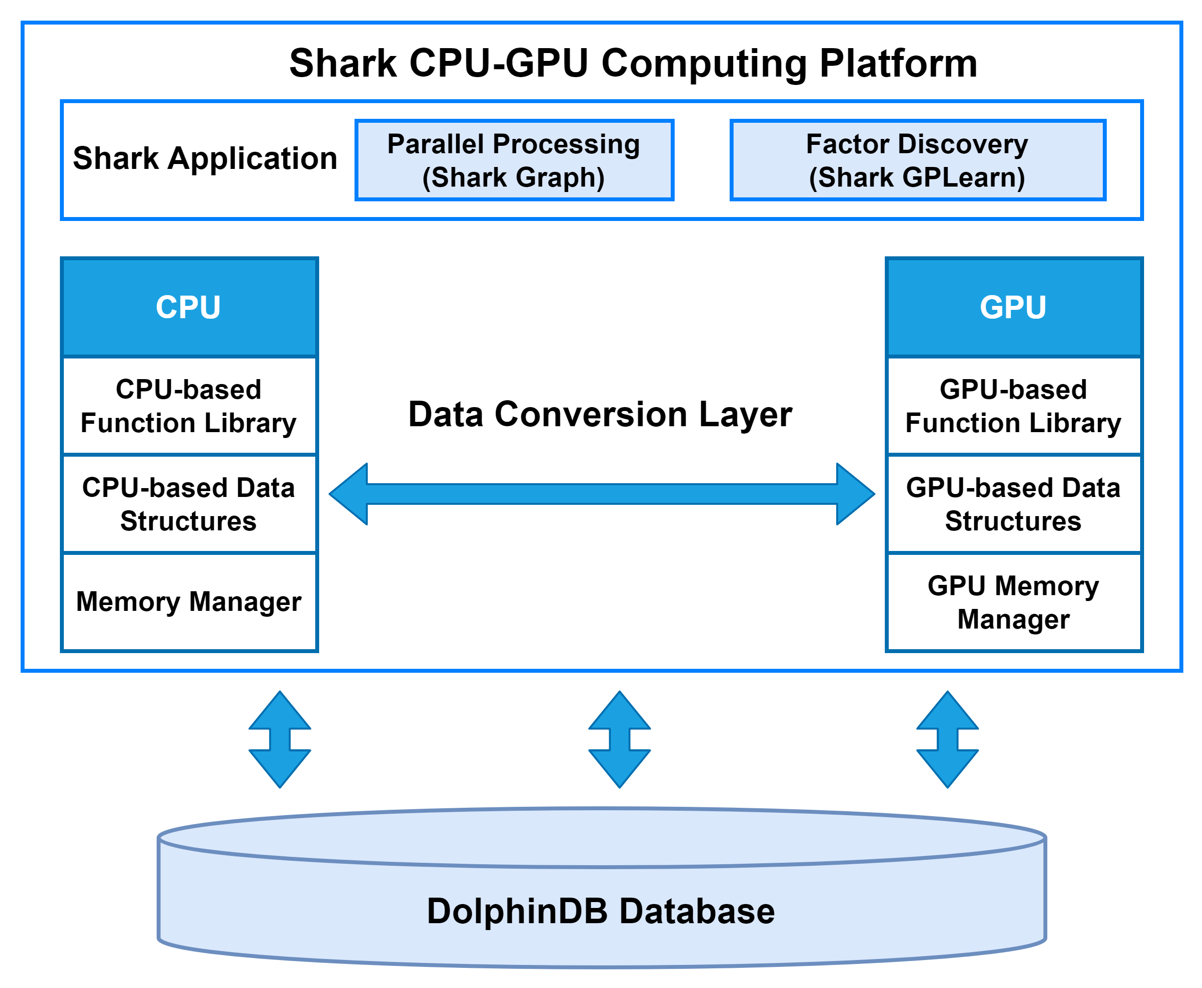
Shark is a CPU–GPU heterogeneous computing platform introduced in DolphinDB 3.0. Built on DolphinDB’s high-performance storage system, Shark deeply integrates GPU parallel computing power to deliver significant acceleration for compute-intensive workloads. Based on a heterogeneous computing framework, Shark consists of two core components:
-
Shark Graph: Accelerates the execution of DolphinDB scripts with GPU parallelism, enabling efficient parallel processing of complex analytical tasks.
-
Shark GPLearn: Designed for quantitative factor discovery, it supports automated factor discovery and optimization based on genetic algorithms.
By leveraging these capabilities, Shark effectively overcomes the performance limitations of traditional CPU computation and greatly enhances DolphinDB’s efficiency in large-scale data analytics, such as high-frequency trading and real-time risk management.
2. Shark GPLearn
2.1 Function Overview
Shark GPLearn is a high-performance module for quantitative factor discovery based on Shark. It can directly read data from DolphinDB and leverage GPUs for automated factor discovery and computation, improving research and investment efficiency.
Compared to Python GPLearn, Shark GPLearn offers a more extensive operator library, including operators for three-dimensional data, along with efficient GPU implementations. Shark introduces group semantics, enabling group-based computations during factor discovery. For mid- and high-frequency raw features such as snapshot and minute-level data, Shark can also perform factor discovery at minute-level and daily frequencies. Additionally, to fully leverage GPU performance, Shark supports multi-GPU on a single machine for genetic algorithm-based factor discovery. For a detailed list of supported operators in Shark, please refer to Quick Start Guide for Shark GPLearn.
2.2 Workflow
Shark GPLearn consists of two main modules: GPLearnEngine and GPExecutor. Its basic architecture is shown below:
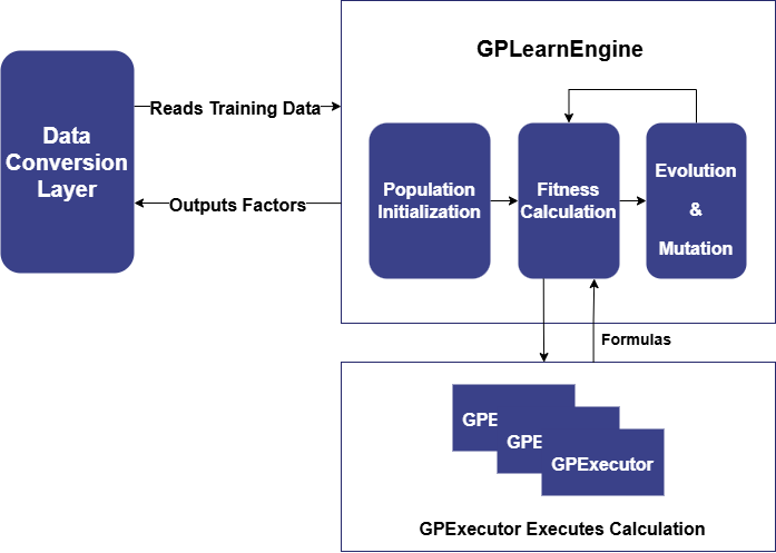
GPLearnEngine is primarily responsible for scheduling tasks during training, including population generation, evolution, and mutation operations. During initialization, GPLearnEngine generates an initial population of formulas and uses a predefined objective function to evaluate how well these formulas align with the given data. Different fitness functions can be used for different applications: for example, in regression problems, the mean squared error between the target value and the formula result can be used, while for quantization factors generated by the genetic algorithm, factor IC can be used as the fitness function.
Subsequently, GPLearnEngine selects suitable formulas from this population based on their fitness, to serve as parents for the next generation's evolution. These selected formulas undergo various evolutionary processes, including Crossover Mutation, Subtree Mutation, Hoist Mutation, and Point Mutation.
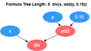
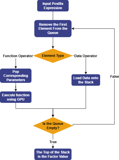
GPExecutor is primarily responsible for calculating the fitness of the
discovered factors. First, it converts the binary tree into a postfix expression
(Reverse Polish Notation). For example, the formula div(x, add(y,
0.15)) will be converted into the form [0.15, y, add, x,
div]. The reverse of this expression forms the execution queue of
the factor, where the variables and constants in the queue are referred to as
data operators, and the functions in the queue are referred to as function
operators.
Subsequently, GPExecutor will traverse the execution queue in order. For data operators, GPExecutor will load the corresponding data onto the stack; for function operators, it will pop the appropriate parameters from the stack based on the function's arguments, then use the GPU to execute the corresponding function, and push the final result back onto the stack. Eventually, the elements in the stack represent the factor values. Once the factor values are obtained, GPExecutor will call the fitness function and calculate the fitness with the predicted data.
Currently, Shark GPLearn also supports downsampled factor discovery. When creating the engine, the aggregation columns can be specified by parameters. During model training, the data will be grouped by aggregation columns, and aggregation functions will be randomly selected for calculations. In downsampled factor discovery, Shark applies constraints to operators through function signatures, thereby automatically generating factor expressions that include downsampled factors, which are evaluated by GPExecutor.
2.3 Quick Start: Symbolic Regression
For a quick deployment of the test environment, please refer to Chapter 4 of Quick Start Guide for Shark GPLearn.
Symbolic regression is a machine learning method that automatically discovers the mathematical expression or function of a given dataset without assuming the specific form of the function. The core of symbolic regression lies in applying a search algorithm to predefine the objective function, finding the optimal expression within the possible mathematical expression space that best fits the data. Symbolic regression is primarily implemented using Genetic Programming (GP).
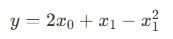
To help beginners get started with Shark GPLearn for factor discovery, this tutorial provides a symbolic regression scenario. Assume the target function is in the following form:
First, simulate the training features (trainData) and regression target (targetData):
// Target function form
def targetFunc(x0, x1){
    return mul(x0,2)+x1-pow(x1,2)
}

// Simulated data: Construct a grid of coordinates where x0 ∈ [-1, 1], x1 ∈ [-1, 1]
x = round(-1 + 0..20*0.1, 1)
x0 = take(x, size(x)*size(x))
x1 = sort(x0)
trainData = table(x0, x1)
targetData = targetFunc(x0, x1)
Create the Shark GPLearn engine, set the fitness function, mutation probabilities, and other related parameters, execute the symbolic regression task, and return the optimal mathematical expression based on fitness.
// Create GPLearnEngine engine
engine = createGPLearnEngine(
trainData, // Independent variables
targetData, // Dependent variables
populationSize=1000, // Population size per generation
generations=20, // Number of generations
stoppingCriteria=0.01, // Fitness threshold for early stopping
tournamentSize=20, // Tournament size, number of competing formulas for the next generation
functionSet=["add", "sub", "mul", "div", "sqrt", "log", "reciprocal", "pow"], // Function set
fitnessFunc="mse", // Fitness function, options: ["mse","rmse","pearson","spearman","mae"]
initMethod="half", // Formula tree initialization method
initDepth=[1, 4], // Formula tree depth range for initialization
restrictDepth=true, // Whether to strictly limit the formula length
constRange=[0, 2.0], // Range of constants in the formula, 0 means no constants
seed=123, // Random seed
parsimonyCoefficient=0.01, // Penalty coefficient for formula complexity
crossoverMutationProb=0.8, // Crossover mutation probability
subtreeMutationProb=0.1, // Subtree mutation probability
hoistMutationProb=0.0, // Hoist mutation probability
pointMutationProb=0.1, // Point mutation probability
minimize=true, // Whether to evolve toward minimum fitness
deviceId=0, // Device ID to use
verbose=true // Whether to output training information
)
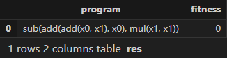
// Get the optimal formula based on fitness
res = engine.gpFit(1) // Result table of Shark GPLearn
resThe expression and fitness result table returned by Shark GPLearn is as follows. As shown, Shark GPLearn has perfectly fitted the target function:
3. Application
3.1 Daily Factor Discovery
3.1.1 Data Preparation
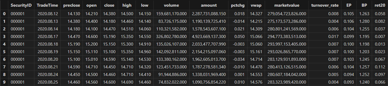
First, use DolphinDB's loadText function to load the daily
market data (DailyOHLC.csv in the Appendix) and split it into training and test data sets. The
training set includes all trading days from August 12, 2020 to December 31,
2022, and the test set includes all trading days from January 1, 2023 to
June 19, 2023.
def processData(splitDay=2022.12.31){
    // Data source: Here we choose to read from a CSV file, the file path should be modified according to the your actual situation
    fileDir = "/home/fln/DolphinDB_V3.00.4/demoData/DailyOHLC.csv"
    colNames = ["SecurityID","TradeDate","ret20","preclose","open","close","high","low","volume","amount","vwap","marketvalue","turnover_rate","pctchg","PE","PB"]
    colTypes = ["SYMBOL","DATE","DOUBLE","DOUBLE","DOUBLE","DOUBLE","DOUBLE","DOUBLE","INT","DOUBLE","DOUBLE","DOUBLE","DOUBLE","DOUBLE","DOUBLE","DOUBLE"]
    t = loadText(fileDir, schema=table(colNames, colTypes))
    // Get training features: Training features need to be FLOAT / DOUBLE types; recommended to sort the training data according to grouping columns
    data =
        select SecurityID, TradeDate as TradeTime,
                preclose,                   // Previous close
                open,                       // Opening price
                close,                      // Closing price
                high,                       // Highest price
                low,                        // Lowest price
                double(volume) as volume,   // Trading volume
                amount,                     // Trading value
                pctchg,                     // Percentage change
                vwap,                       // Volume-Weighted Average Price (VWAP)
                marketvalue,                // Market value
                turnover_rate,              // Turnover rate
                double(1\PE) as EP,         // Earnings yield
                double(1\PB) as BP,         // Price-to-book ratio
                ret20                       // 20-day future return rate
        from t order by SecurityID, TradeDate
    // Split into training set
    days = distinct(data["TradeTime"])
    trainDates = days[days<=splitDay]
    trainData = select * from data where TradeTime in trainDates order by SecurityID, TradeTime
    // Split into test set
    testDates = days[days>splitDay]
    testData = select * from data where TradeTime in testDates order by SecurityID, TradeTime
    return data, trainData, testData
}

splitDay = 2022.12.31                                   // Split date for training and test set
allData, trainData, testData = processData(splitDay)    // All data set, training set, test set
The table schema of the daily data is shown below:
3.1.2 Model Training
Create the Shark GPLearnEngine. The engine provides a variety of parameters for you to configure and modify as needed. For the detailed information on the parameters, refer to the documentation: createGPLearnEngine.
In the following example, parameters such as functionSet, initProgram are configured.
-
functionSet: The operator library used to generate formulas. It can include commonly used sliding window functions.
-
initProgram: The initial population that you can customize.
-
groupCol: Grouping column. When using sliding window functions, grouped calculations are supported.
-
minimize: Whether to minimize. It allows you to specify the direction of evolution.
-
parsimonyCoefficient: Penalty coefficient. It can limit the length of formulas.
trainX = dropColumns!(trainData.copy(), ["TradeTime", "ret20"])     // Independent variables for training data
trainY = trainData["ret20"]                                         // Dependent variable for training data
trainDate = trainData["TradeTime"]                                  // Time information for training data
// Configure function set
functionSet = ["add", "sub", "mul", "div", "sqrt", "reciprocal", "mprod", "mavg", "msum", "mstdp", "mmin", "mmax", "mimin", "mimax","mcorr", "mrank", "mfirst"]
// Define initial formulas
alphaFactor = {
    // world quant 101
    "wqalpha6":<-1 * mcorr(open, volume, 10)>,
    "wqalpha12":<signum(deltas(volume)) * (-1 * deltas(close))>,
    "wqalpha26":<-1 * mmax(mcorr(mrank(volume, true, 5), mrank(high, true, 5), 5), 3)>,
    "wqalpha35":<mrank(volume, true, 32) * (1 - mrank((close + high - low), true, 16)) * (1 - mrank((ratios(close) - 1), true, 32))>,
    "wqalpha43":<mrank(div(volume, mavg(volume, 20)), true, 20) * mrank(-1*(close - mfirst(close, 8)), true, 8)>,
    "wqalpha53":<-1 * (div(((close - low) - (high - close)), (close - low)) - mfirst(div(((close - low) - (high - close)), (close - low)), 10))>,
    "wqalpha54":<-1 * div((low - close) * pow(open, 5), (low - high) * pow(close, 5))>,
    "wqalpha101":<div(close - open, high - low + 0.001)>,
    // Guotai Juan Alpha 191
    "gtjaAlpha2":<-1 * deltas(div(((close - low) - (high - close)), (high - low)))>,
    "gtjaAlpha5":<-1 * mmax(mcorr(mrank(volume, true, 5), mrank(high, true, 5), 5), 3)>,
    "gtjaAlpha11":<msum(div((close - low - (high - close)),(high - low)) * volume, 6)>,
    "gtjaAlpha14":<close - mfirst(close, 6)>,
    "gtjaAlpha15":<deltas(open) - 1>,
    "gtjaAlpha18":<div(close, mfirst(close, 6))>,
    "gtjaAlpha20":<div(close - mfirst(close, 7), mfirst(close, 7)) * 100>
}
initProgram = take(alphaFactor.values(), 600) // Initial population

// Create GPLearnEngine engine
engine = createGPLearnEngine(trainX,trainY,    // Training data
                       groupCol="SecurityID",  // Grouping column: group by SecurityID for sliding window
                       seed=42,             // Random seed
                       populationSize=1000, // Population size
                       generations=10,      // Number of generations
                       tournamentSize=20,   // Tournament size, number of formulas competing for the next generation
                       functionSet=functionSet, // Function set
                       initProgram=initProgram, // Initial population
                       minimize=false,          // false means maximizing fitness
                       initMethod="half",        // Initialization method
                       initDepth=[2, 4],        // Initial formula tree depth range
                       restrictDepth=true,      // Whether to strictly limit the tree depth
                       windowRange=[5,10,20,40,60], // Window range
                       constRange=0,             // 0 means no constants in the formula
                       parsimonyCoefficient=0.05,// Complexity penalty coefficient
                       crossoverMutationProb=0.6,// Crossover mutation probability
                       subtreeMutationProb=0.01, // Subtree mutation probability
                       hoistMutationProb=0.01,   // Hoist mutation probability
                       pointMutationProb=0.01,   // Point mutation probability
                       deviceId=0                // Device ID
                       )
The parsimonyCoefficient parameter is used to constrain the length of the formula tree by applying a penalty to the fitness score during evaluation, as defined by the following formula:

Where:
-
rawfitness indicates the original fitness,
-
parsimony indicates the parsimony coefficient,
-
length indicates the length of the formula tree,
-
sign indicates the direction of fitness evolution. If the fitness evolution direction is positive, its value is 1; if negative, its value is -1.
In Shark:
-
When minimizing fitness as the objective, a positive parsimony coefficient encourages shorter formula trees, while a negative parsimony coefficient encourages longer formula trees.
-
When maximizing fitness as the objective, a positive parsimony coefficient encourages longer formula trees, while a negative parsimony coefficient encourages shorter formula trees.
In factor discovery, based on the financial attributes of the factors, we can set rankIC as the fitness function to guide the model in discovering factor formulas that have a higher correlation with returns. Specifically, we set the model's fitness function as the mean RankIC calculated per date from the factor values produced during training. The formula is as follows:
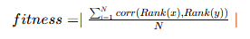
Where N is the number of groups, corresponding to the number of trading days
in the training set. The custom fitness function, along with the date
grouping column, is passed to GPLearnEngine via
setGpFitnessFunc. Currently, DolphinDB supports adding
helper operators such as groupby,
contextby, rank,
zscore, etc., in the custom fitness function. For the
complete list of helper operators, refer to the setGpFitnessFunc function documentation.
// Modify the fitness function to a customized function: calculate Rank IC
def myFitness(x, y, groupCol){
return abs(mean(groupby(spearmanr, [x, y], groupCol)))
}
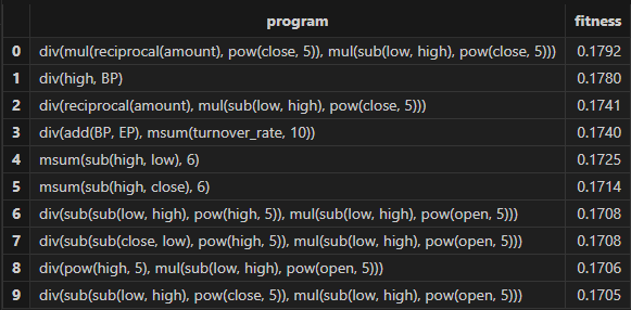
setGpFitnessFunc(engine, myFitness, trainDate)Once the model is configured, you can call the gpFit
function for model training and return the top programNum factor formulas
based on fitness.
// Train the model to discover factors
programNum=30
timer res = engine.gpFit(programNum)
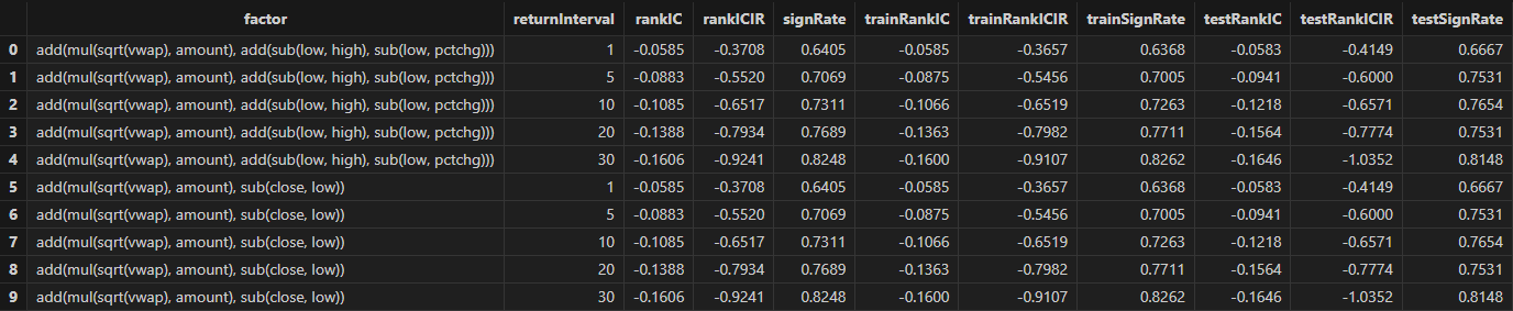
// View the discovery results
resThe factor results with better fitness returned by Shark GPLearn are shown in the table below:
3.1.3 Factor Evaluation
Once model training is complete, you can use the gpPredict
function to calculate factor values.
allX = dropColumns!(allData.copy(), ["TradeTime", "ret20"])         // Independent variables for all data
// Calculate all factor values
factorValues = gpPredict(engine, allX, programNum=programNum, groupCol="SecurityID")
factorList = factorValues.colNames()                                // Factor list
totalData = table(allData, factorValues)
This tutorial uses DolphinDB's alphalens module (Application of Alphalens in DolphinDB: Practical Factor Analysis Modeling) to develop the single-factor evaluation function.
The single-factor evaluation function in this tutorial has been modified as follows:
-
Data Preprocessing:
-
Standardize the factor values using Z-score.
-
Call the
get_clean_factor_and_forward_returnsfunction from Alphalens to calculate future returns over different periods and group factor values by quantiles.
-
-
IC Method:
-
Call the
factor_information_coefficientfunction from Alphalens to calculate daily rankIC of the factor.
-
-
Stratified Backtesting:
-
Manually adjust factor groups for the holding period. For example, if the holding period is 5, the factor groups for the next 4 days are based on the group from the first day.
-
Call the
mean_return_by_quantilefunction from Alphalens to calculate the average return for each group over different future periods. -
Call the
plot_cumulative_returns_by_quantilefunction from Alphalens to convert the average returns into cumulative returns, providing a visual comparison of the long-term performance and differentiation of different quantile combinations.
-
Here's the specific code:
/*
Custom single-factor evaluation function
@params:
totalData: Factor data
factorName: Factor name, used to query the specific factor values from totalData
priceData: Price data, used to calculate factor returns
returnIntervals: List of holding periods
quantiles: Quantile divisions, used for factor stratification
*/
def singleFactorAnalysis(totalData, factorName, priceData, returnIntervals, quantiles){
print("factorName: "+factorName+" analysis start")
/* Data preprocessing: calculate future returns for different periods and group factor values */
// Extract the factor values and standardize them
factorVal = eval(<select TradeTime as date, SecurityID as asset, zscore(_$factorName) as factor from totalData context by TradeTime>)
// Call alphalens's get_clean_factor_and_forward_returns function to calculate future returns for different periods, and group factor values by quantiles to generate intermediate analysis results.
periods = distinct(returnIntervals<-[1]).sort()
cleanFactorAndForwardReturns = alphalens::get_clean_factor_and_forward_returns(
factor=factorVal, // Factor data
prices=priceData, // Price data
quantiles=quantiles, // Quantile divisions
periods=periods, // Future return periods
max_loss=0.1, // Maximum data loss tolerance. During data cleaning, invalid data (e.g., NaN factors or missing returns) may be discarded.
// This parameter sets a ratio (e.g., 0.1 means 10%). If the discarded data exceeds this proportion, the function will throw an error. Set to 0 to allow no data discard.
cumulative_returns=true // Whether to compute cumulative returns for multiple periods
)
/* IC Method for factor evaluation */
// Call alphalens's factor_information_coefficient function to calculate the rankIC for each day
factorRankIC = select factorName as `factor, * from alphalens::factor_information_coefficient(cleanFactorAndForwardReturns)
factorRankIC = select factor, date, int(each(last, valueType.split("_"))) as returnInterval, value as rankIC
from unpivot(factorRankIC, keyColNames=`factor`date, valueColNames=factorRankIC.colNames()[2:])
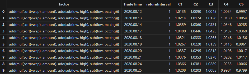
/* Stratified Backtesting for factor evaluation */
// Get all backtest time
timeList = sort(distinct(totalData["TradeTime"]))
// Get the data for stratified backtesting
sliceData = select date, asset, forward_returns_1D, factor_quantile, factor_quantile as periodGroup from cleanFactorAndForwardReturns
// Construct the function for grouping backtest by holding period
quantileTestFun = def(timeList, sliceData, returnInterval){
// Assign holding period groups to each backtest time point based on the holding period
periodDict = dict(timeList, til(size(timeList))/returnInterval)
// Replace group information within the period based on holding period (e.g., for holding period 5, the factor groups for the next 4 days follow the first day's group)
update sliceData set factor_quantile = periodGroup[0] context by asset, periodDict[date]
tmp = select * from sliceData where factor_quantile!=NULL
ret, stdDaily = alphalens::mean_return_by_quantile(sliceData, by_date=true, demeaned=false)
ret = alphalens::plot_cumulative_returns_by_quantile(ret, period="forward_returns_1D")
// Adjust the result table
groupCols = sort(ret.colNames()[1:])
res = eval(<select date as `TradeTime, returnInterval as `returnInterval, _$$groupCols as _$$groupCols from ret order by date>)
return res
}
// Calculate stratified backtest results for different holding periods
quantileRes = select factorName as `factor, * from each(quantileTestFun{timeList, sliceData}, returnIntervals).unionAll()
print("factorName:"+factorName+"analysis finished")
return factorRankIC, quantileRes
}You can apply the custom single-factor evaluation function to each factor
discovered by Shark GPLearnEngine in batch using the peach
function. The final results will include:
-
rankICRes: The RankIC series of each factor across different future return intervals.
-
quantileRes: The performance of return intervals at each time point after grouping factors by quantiles.
-
rankICStats: Statistical metrics on the training set, test set, and full data set, including the RankIC mean, RankIC IR, and the proportion of RankIC values that align with the direction of the RankIC mean.
/*
    Batch Backtesting for Factors
    @params:
        totalData: Factor data
        factorName: Factor list
        returnIntervals: Holding period list
        quantiles: Quantile divisions
        splitDay: The split date for the training and test sets
*/
def analysisFactors(totalData, factorList, returnIntervals, quantiles=5, splitDay=2022.12.31){
    // Retrieve the price data for each time
    priceData = select close from totalData pivot by TradeTime as date, SecurityID
    // Single factor evaluation
    resDataList = peach(singleFactorAnalysis{totalData, , priceData, returnIntervals, quantiles}, factorList)
    // Summary of results
    rankICRes = unionAll(resDataList[, 0], false)
    quantileRes = unionAll(resDataList[, 1], false)
    // Analyze rankIC results for all data
    calICRate = defg(rankIC){return sum(signum(avg(rankIC))*rankIC > 0) \ count(rankIC)}
    allRankIC = select  avg(rankIC) as rankIC,
                        avg(rankIC) \ stdp(rankIC) as rankICIR,
                        calICRate(rankIC) as signRate
                from rankICRes group by factor, returnInterval
    // Analyze rankIC results for training set
    trainRankIC = select avg(rankIC) as trainRankIC,
                         avg(rankIC) \ stdp(rankIC) as trainRankICIR,
                         calICRate(rankIC) as trainSignRate
                from rankICRes where date<=splitDay group by factor, returnInterval
    // Analyze rankIC results for test set
    testRankIC = select avg(rankIC) as testRankIC,
                        avg(rankIC) \ stdp(rankIC) as testRankICIR,
                        calICRate(rankIC) as testSignRate
                from rankICRes where date>splitDay group by factor, returnInterval
    // Summary of results
    factor = table(factorList as factor)
    rankICStats = lj(factor, lj(allRankIC, lj(trainRankIC, testRankIC, `factor`returnInterval), `factor`returnInterval), `factor)
    return rankICRes, quantileRes, rankICStats
}

/* Single-factor analysis
rankICRes: View the RankIC details table for factors
quantileRes: View the final stratified return results table
rankICStats: View the RankIC analysis table
*/
rankICRes, quantileRes, rankICStats = analysisFactors(totalData, factorList, returnIntervals=[1,5,10,20,30], quantiles=[0.0, 0.2, 0.4, 0.6, 0.8, 1.0], splitDay=splitDay)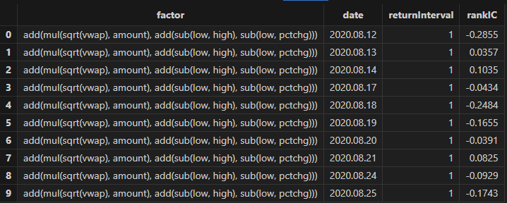
3.1.4 Results Visualization
In this example, we filter factors based on three metrics: RankIC mean, RankICIR absolute value, and IC win rate. The specific filter criteria are as follows:
-
The absolute value of RankIC mean must be at least 0.05.
-
The absolute value of RankICIR must be at least 0.5.
-
The IC win rate must exceed 65%.
Run the following code to obtain the final selected daily factors. You can adjust the filtering rules according to your actual strategy.
// Factor filtering
retInterval = 20                   // Select the holding periods for display
factorPool =
    select * from rankICStats
    where returnInterval=retInterval
        and abs(rankIC)>=0.05 and abs(rankICIR)>=0.5 and signRate>=0.65
        and isDuplicated([round(abs(rankIC), 4), round(abs(rankICIR), 4)])=false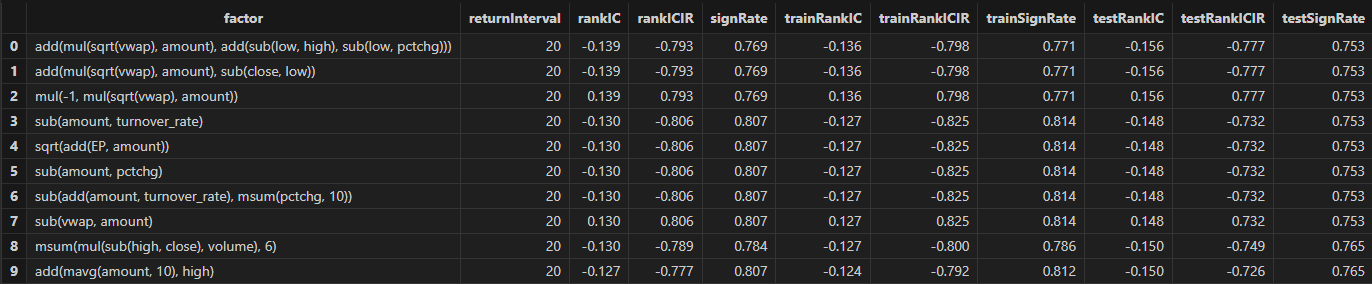
Run the following code to view the daily RankIC and cumulative RankIC results for the selected daily factors returned by Shark GPLearn:
// Visualize daily RankIC and cumulative RankIC
factorName = factorPool[`factor][0]         // Select the factors for display
sliceData = select date, rankIC, cumsum(RankIC) as cumRankIC from rankICRes where factor=factorName and returnInterval=retInterval
plot(sliceData[`rankIC`cumRankIC], sliceData[`date], extras={multiYAxes: true})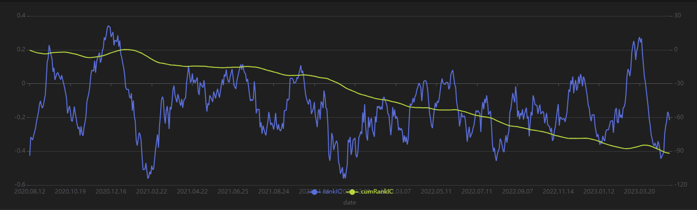
As shown in the above chart, the RankIC performance of the factor is stable both in the training period (before 2023) and the test period (after 2023): for most of the time, the RankIC of the factor remains below zero, and the cumulative RankIC steadily declines.
Run the following code to view the RankIC results for the selected dailyfactors across different return intervals. You can see that this factor demonstrates strong predictive ability for future 1-30 day returns:
// Visualize RankIC Mean
sliceData = select * from rankICStats where factor=factorName
plot(sliceData[`rankIC`trainRankIC`testRankIC], sliceData[`returnInterval])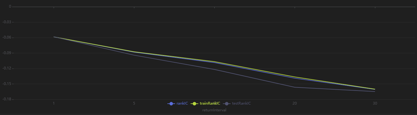
Run the following code to view the stratified return results for every 20 trading days, grouped by the factor value on the first day. As shown in Figure 3-9, the stratified backtest results align with the IC method results—this factor shows a significantly negative IC value when using the future 20-day return interval. Using a 20-day rebalancing interval for the stratified backtest, we find that:
-
The group with the highest factor value (Group 5) has the lowest overall return.
-
The group with the lowest factor value (Group 1) has the highest overall return.
The clear stratification between groups indicates the factor performs well.
// Visualize Stratified Return
sliceData = select * from quantileRes where factor=factorName and returnInterval=retInterval
plot(sliceData[columnNames(sliceData)[3:]],sliceData[`TradeTime]) 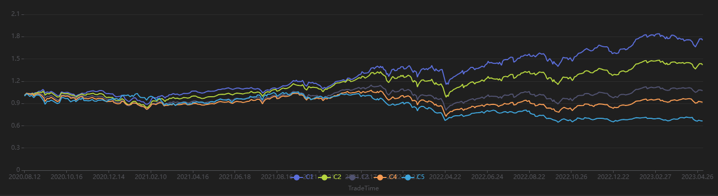
3.2 Minute-Level Factor Discovery
3.2.1 Data Preparation
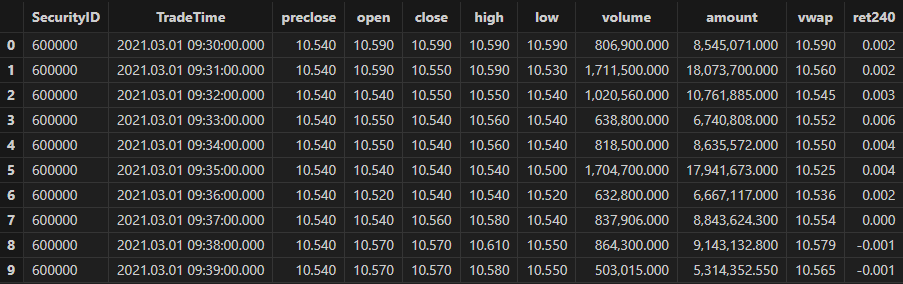
First, use DolphinDB's loadText function to load the
minute-level data (MinuteOHLC.csv in the Appendix) and split it into training and test data sets. The
training set spans from March 1, 2021, to October 31, 2021, and the test set
spans from November 1, 2021, to December 31, 2021.
def processData(splitDay=2021.11.01){
    // Data source: Choose to load from CSV. Modify the file path according to your actual situation.
    fileDir = "/home/fln/DolphinDB_V3.00.4/demoData/MinuteOHLC.csv"
    colNames = ["SecurityID","TradeTime","preclose","open","high","low","close","volume","amount"]
    colTypes = ["SYMBOL","TIMESTAMP","DOUBLE","DOUBLE","DOUBLE","DOUBLE","DOUBLE","INT","DOUBLE"]
    t = loadText(fileDir, schema=table(colNames, colTypes))
    // Get training features: The training features must be of type FLOAT / DOUBLE; the data should be sorted by grouping column.
    data =
        select SecurityID,
                TradeTime,                  // Trade time
                preclose,                   // Previous close
                open,                       // Opening price
                close,                      // Closing price
                high,                       // Highest price
                low,                        // Lowest price
                double(volume) as volume,   // Trading volume
                amount,                     // Trading value
                nullFill(ffill(Amount \ Volume), 0.0) as vwap,// VWAP
                move(close,-241)\close-1 as ret240   // Future 240-minute return
        from t context by SecurityID order by SecurityID, TradeTime
    data = select * from data where not isNull(ret240)
    // Split into training set
    days = distinct(data["TradeTime"])
    trainDates = days[days<=splitDay]
    trainData = select * from data where TradeTime in trainDates order by SecurityID, TradeTime
    // Split into test set
    testDates = days[days>splitDay]
    testData = select * from data where TradeTime in testDates order by SecurityID, TradeTime
    return data, trainData, testData
}

splitDay = 2021.11.01                                   // Split date for training and test set
allData, trainData, testData = processData(splitDay)    // All data set, training set, test set
Table schema for minute-level data:
3.2.2 Model Training
Similar to the case for daily scenario, create the Shark GPLearnEngine first. Since Alpha 101 and Alpha 191 are designed for daily factors, they may not be effective in the minute-level scenario. Therefore, the initProgram parameter is not set, and Shark directly generates the specified number of initial populations. For the fitness function, we use Shark's built-in Spearman correlation coefficient for calculation.
trainX = dropColumns!(trainData.copy(), ["TradeTime", "ret240"]) // Independent variables for training data
trainY = trainData["ret240"] // Dependent variable for training data
trainDate = trainData["TradeTime"] // Time information for training data
// Configure the function set
functionSet = ["add", "sub", "mul", "div", "sqrt", "reciprocal", "mavg", "msum", "mstdp", "mmin", "mmax", "mimin", "mimax","mcorr", "mrank", "mfirst"]
// Create GPLearnEngine
engine = createGPLearnEngine(trainX,trainY, // Training data
fitnessFunc="spearmanr", // Fitness function
groupCol="SecurityID", // Group column: Group by SecurityID for sliding window
seed=42, // Random seed
populationSize=1000, // Population size
generations=5, // Number of generations
tournamentSize=20, // Tournament size: Number of formulas competing for the next generation
functionSet=functionSet, // Function set
initProgram=NULL, // Initial population
minimize=false, // false indicates maximize the fitness
initMethod="half", // Initialization method
initDepth=[3, 5], // Initial formula tree depth range
restrictDepth=true, // Whether to strictly limit the depth of the tree
windowRange=[30,60,120,240,480], // Window range
constRange=0, // 0 means no extra constants generated in the formula
parsimonyCoefficient=0.8, // Parsimony coefficient
crossoverMutationProb=0.8,
subtreeMutationProb=0.1,
hoistMutationProb=0.02,
pointMutationProb=0.02,
deviceId=0 // Specify the device ID
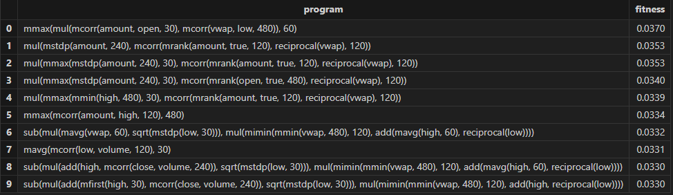
)After configuring the model, call the gpFit function to
train the model and return the top programNum factor formulas based on
fitness.
// Train the model and discover the factors
programNum=30
timer res = engine.gpFit(programNum)
// View the results
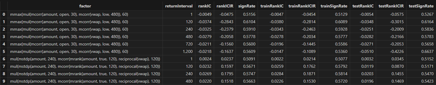
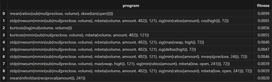
resThen Shark GPLearn returns the factor results with higher fitness as shown in the table below:
3.2.3 Factor Evaluation
After training the model, you can use the gpPredict function
to calculate the factor values.
allX = dropColumns!(allData.copy(), ["TradeTime", "ret240"])         // Independent variables for all data
// Calculate all factor values
factorValues = gpPredict(engine, allX, programNum=programNum, groupCol="SecurityID")
factorList = factorValues.colNames()                                // Factor list
totalData = table(allData, factorValues)
Use the single-factor evaluation function from Section 3.1.3 to execute factor evaluation and view the results:
/* Single Factor Analysis
rankICRes: View the detailed rankIC table for factors
quantileRes: View the final results table for stratified returns
rankICStats: View the rankIC analysis table
*/
// Single Factor Analysis
rankICRes, quantileRes, rankICStats = analysisFactors(totalData, factorList, returnIntervals=[120, 240, 480, 720, 1200], quantiles=[0.0, 0.2, 0.4, 0.6, 0.8, 1.0], splitDay=splitDay)
3.2.4 Results Visualization
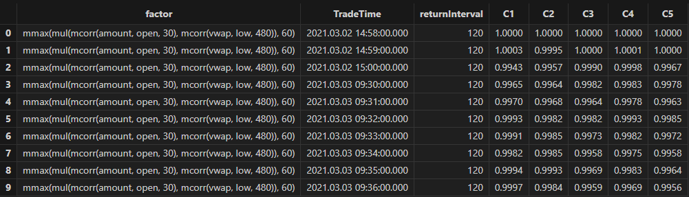
Run the following code to view the minute-level RankIC and cumulative RankIC results for the selected minute-level factor returned by Shark GPLearn:
// Visualize minute-level RankIC and cumulative RankIC
factorName = factorList[0]         // Select the factors to display
retInterval = 240                  // Select the holding periods for display
sliceData = select date, rankIC, cumsum(RankIC) as cumRankIC from rankICRes where factor=factorName and returnInterval=retInterval
plot(sliceData[`rankIC`cumRankIC], sliceData[`date], extras={multiYAxes: true})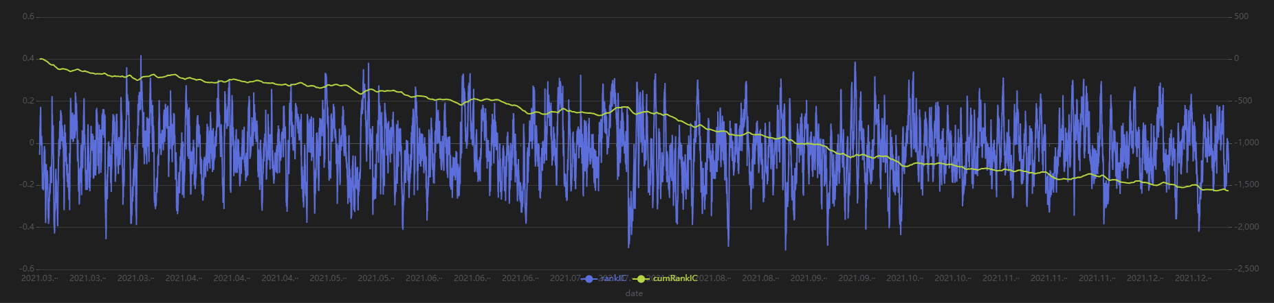
As shown in the above chart, the RankIC of this minute-level factor is mostly less than 0, and the cumulative RankIC steadily declines, indicating that this factor has a good predictive effect on future 240-minute return.
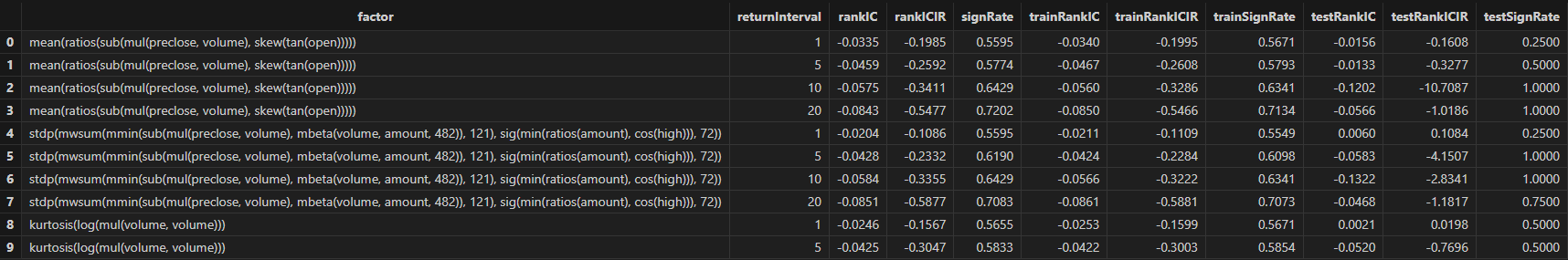
Run the following code to view the RankIC results for the selected minute-level factor at different return intervals:
// Visualize RankIC mean
sliceData = select * from rankICStats where factor=factorName
plot(sliceData[`rankIC`trainRankIC`testRankIC], sliceData[`returnInterval])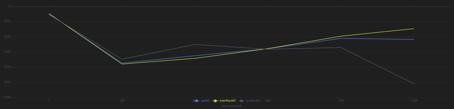
As shown in the above chart, across all sample intervals, this factor predicts future 120-minute and 240-minute returns more effectively than other intervals.
Run the following code to view the stratified return results for a 240-minute holding period, grouped by the first minute’s factor value. The final stratified returns show a ranking from 1 to 5, consistent with the negative RankIC result, indicating that this factor performs well in terms of stratified returns for the 240-minute rebalancing interval:
// Visualize stratified returns
sliceData = select * from quantileRes where factor=factorName and returnInterval=retInterval
plot(sliceData[columnNames(sliceData)[3:]],sliceData[`TradeTime]) 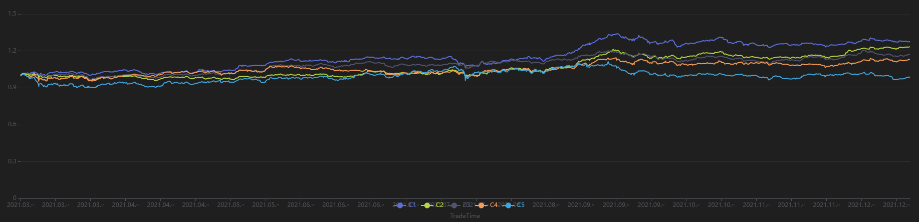
3.3 Downsampled Factor Discovery
This section uses minute-level OHLC as training data. The security and date columns are used as downsampling columns. The target for training is the future 20-day return of individual stocks at daily level. And the goal is to perform downsampled factor discovery from minute-level inputs to daily outputs.
3.3.1 Data Preparation
First, use the same data used for minute-level factor discovery and applying downsampling to obtain dailyfactor results. Then, perform factor evaluation and visualization. The training set spansfrom March 1, 2021 to October 31, 2021, and the test set spans from November 1, 2021 to December 31, 2021.
def processData(splitDay=2021.11.01){
    // Data source: Choose to read from CSV, modify the file path as needed
    fileDir = "/home/fln/DolphinDB_V3.00.4/demoData/MinuteOHLC.csv"
    colNames = ["SecurityID","TradeTime","preclose","open","high","low","close","volume","amount"]
    colTypes = ["SYMBOL","TIMESTAMP","DOUBLE","DOUBLE","DOUBLE","DOUBLE","DOUBLE","INT","DOUBLE"]
    t = loadText(fileDir, schema=table(colNames, colTypes))
    // Get training features: Training features must be of FLOAT / DOUBLE type; it is also recommended to sort training data by group column
    data =
        select SecurityID,
                date(TradeTime) as TradeDate, // Trade date
                TradeTime,                  // Trade time
                preclose,                   // Previous close
                open,                       // Opening price
                close,                      // Closing price
                high,                       // Highest price
                low,                        // Lowest price
                double(volume) as volume,   // Trading volume
                amount,                     // Trading value
                nullFill(ffill(Amount \ Volume), 0.0) as vwap,// VWAP
                move(close,-241*20)\close-1 as ret20   // Future 20-day return
        from t context by SecurityID order by SecurityID, TradeTime
    data = select * from data where ret20!=NULL order by SecurityID, TradeTime
    // Split into training set
    days = distinct(data["TradeTime"])
    trainDates = days[days<=splitDay]
    trainData = select * from data where TradeTime in trainDates order by SecurityID, TradeTime
    // Split into test set
    testDates = days[days>splitDay]
    testData = select * from data where TradeTime in testDates order by SecurityID, TradeTime
    return data, trainData, testData
}
splitDay = 2021.11.01                                   // Split date for training and test set
allData, trainData, testData = processData(splitDay)    // All data set, training set, test set
3.3.2 Model Training
Unlike the minute-level and daily scenarios, this case involves a change in both input and output data frequencies. So it is necessary to specify the downsampling columns in advance and pass the downsampled target variable column into the Shark GPLearn Engine. Note that the input target variable is the downsampled result. Therefore, the vector length of the input targetData must match the number of groups produced by aggregating the trainData according to the downsampling column. Below is the code for downsampled factor discovery:
// Minute-level data input
trainX = dropColumns!(trainData.copy(),`ret20`TradeTime)
// Daily output
trainDailyData = select last(ret20) as `ret20 from trainData group by SecurityID, TradeDate
trainY = trainDailyData["ret20"]
trainDate = trainDailyData["TradeDate"]                                  // Training data time information
// Create GPLearnEngine
engine = createGPLearnEngine(trainX,trainY,    // Training data
                       fitnessFunc="spearmanr", // Fitness function
                       dimReduceCol=["SecurityID", "TradeDate"], // Downsampling columns: downsample by TradeDate column
                       groupCol="SecurityID",  // Grouping column: slide by SecurityID
                       seed=999,             // Random seed
                       populationSize=1000, // Population size
                       generations=4,      // Number of generations
                       tournamentSize=20,   // Tournament size, number of formulas competing for the next generation
                       minimize=false,          // false means maximize the fitness
                       initMethod="half",        // Initialization method
                       initDepth=[3, 6],        // Initial formula tree depth
                       restrictDepth=true,      // Whether to strictly limit tree depth
                       windowRange=int([0.1, 0.2, 0.3, 0.4, 0.5, 0.8, 1, 2, 5]*241), // Window range
                       constRange=0,             // 0 means no extra constants in the formula
                       parsimonyCoefficient=0.8, // Parsimony coefficient
                       crossoverMutationProb=0.8,
                       subtreeMutationProb=0.1,
                       hoistMutationProb=0.02,
                       pointMutationProb=0.02,
                       deviceId=0                // Specify the device ID
                       )
After model configuration, call gpFit function for model
training and return the factor formulas based on fitness.
// Train the model for factor discovery
programNum = 20
timer res = engine.gpFit(programNum)
// View the results
res
Then Shark GPLearn returns the factor result table with higher fitness, as shown below:
3.3.3 Factor Evaluation
After model training, use the gpPredict function for factor
calculation. For downsampled factors, specify the dimReduceCol in
gpPredict, which corresponds to the downsampling column
parameter used during training.
Note that the number of rows output by gpPredict is the same
as the input data, not the final downsampled result. In fact, only the first
n rows are valid, where n equals the final number of groups. Therefore, in
the following code, the output of gpPredict should be
sliced using [0: rows(totalData)] to obtain the downsampled factor
results.
allX = dropColumns!(allData.copy(), ["TradeTime", "ret20"])         // Independent variables for all data
// Calculate all factor values
factorValues = select * from gpPredict(engine, allX, programNum=programNum, groupCol="SecurityID", dimReduceCol=["SecurityID", "TradeDate"])
factorList = factorValues.colNames()                                // Factor list
// Output daily results
totalData = select last(close) as close from allData group by SecurityID, TradeDate as TradeTime
totalData = table(totalData, factorValues[0:rows(totalData), ])
Use the single-factor evaluation function from Section 3.1.3 to execute the factor evaluation and view the results:
/* Single-factor analysis
    rankICRes: View the detailed factor rankIC table
    quantileRes: View the final quantile return results table
    rankICStats: View the rankIC analysis table
*/
rankICRes, quantileRes, rankICStats = analysisFactors(totalData, factorList, returnIntervals=[1,5,10,20], quantiles=[0.0, 0.2, 0.4, 0.6, 0.8, 1.0], splitDay=splitDay)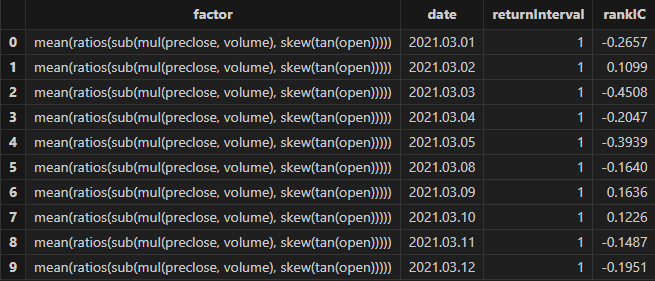

3.3.4 Results Visualization
Run the following code to visualize the dailyRankIC and cumulative RankIC of the selected downsampled factors returned by Shark GPLearn:
// Visualize daily RankIC and cumulative RankIC
factorName = factorList[0]         // Select the factors to display
retInterval = 20                  // Select the holding period to display
sliceData = select date, rankIC, cumsum(RankIC) as cumRankIC from rankICRes where factor=factorName and returnInterval=retInterval
plot(sliceData[`rankIC`cumRankIC], sliceData[`date], extras={multiYAxes: true})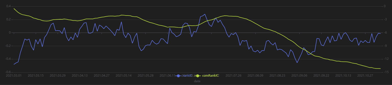
As shown in the above chart, the RankIC of this factor is mostly less than 0 during the period, and the cumulative RankIC steadily declines. This suggests that the factor has good predictive power for the future 20-day returns.
Run the following code to view the RankIC results for different future return intervals (1-30 days) of the selected factor returned by Shark GPLearn. It shows that the factor has good predictive ability for returns across all these intervals:
// Visualize RankIC mean
sliceData = select * from rankICStats where factor=factorName
plot(sliceData[`rankIC`trainRankIC`testRankIC], sliceData[`returnInterval])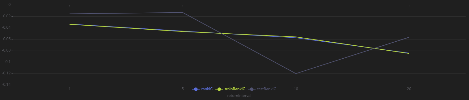
Run the following code to view the stratified returns based on the factor values of the first day, calculated with a 20-day holding period. The stratified backtest results align with the IC method — the factor has a significantly negative IC value using future 20-day returns, and the backtest results show that the highest value group (Group 5) has the lowest returns, while the lowest value group (Group 1) has the highest returns, indicating the factor performs well:
// Visualize stratified returns
sliceData = select * from quantileRes where factor=factorName and returnInterval=retInterval
plot(sliceData[columnNames(sliceData)[3:]],sliceData[`TradeTime]) 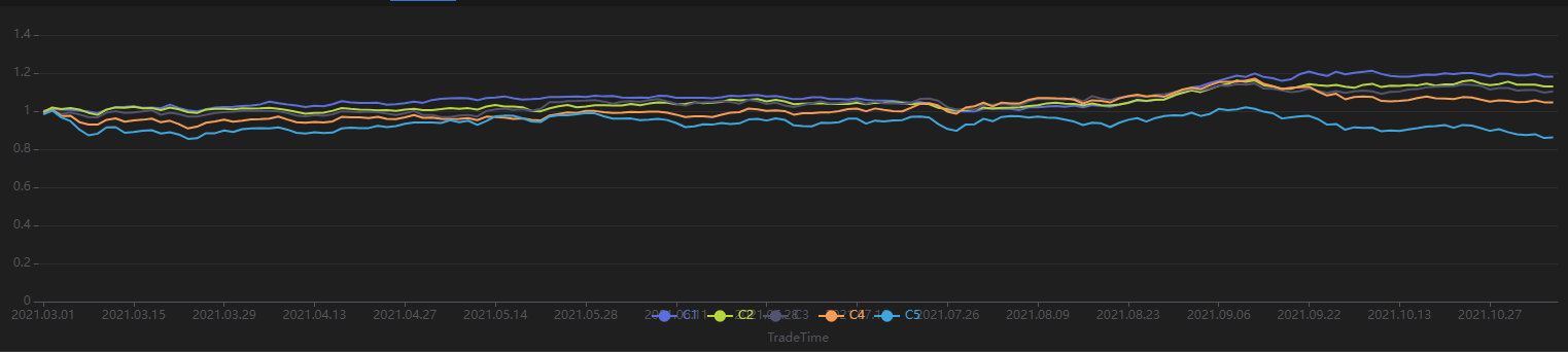
3.4 Advanced: Automated Factor Discovery
3.4.1 Introduction to Automated Factor Discovery Method
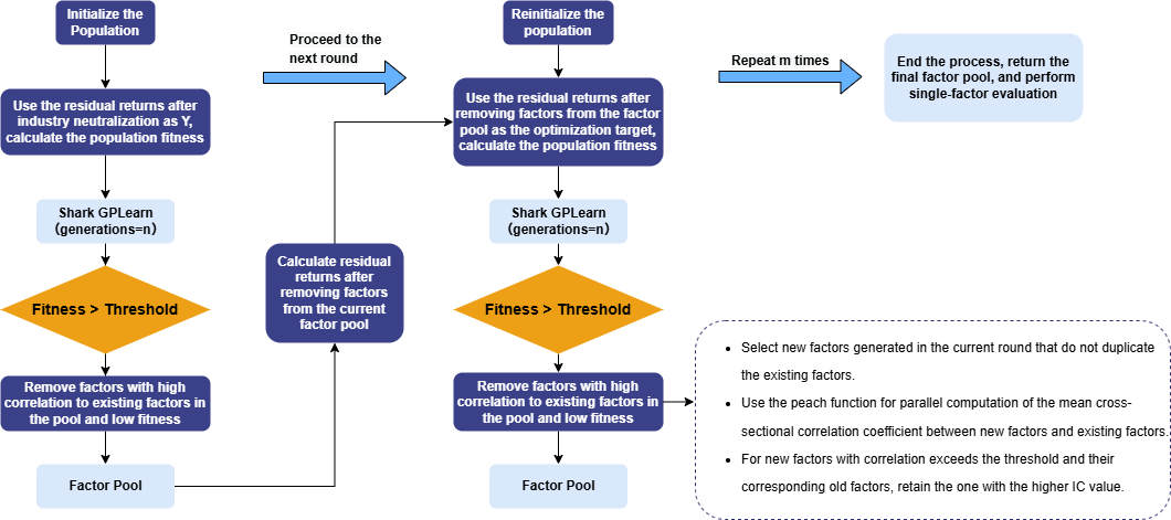
The automated factor discovery method used in this tutorial aims to discover incremental information that explains returns in each round. In the first round of Shark GPLearn factor discovery, the residual returns after removing style factors (such as log market value and industry) are used as the prediction target. The mean of the cross-sectional correlation coefficients between factor values and residual returns is taken as the factor fitness. After the new factors pass the fitness and correlation screening, they are stored, while the old factors being replaced are removed. The new factors discovered in the next round are then used to perform regression and obtain the residual returns for the next round.
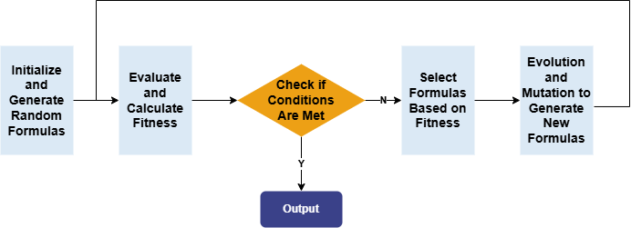
Repeat this process for multiple rounds of factor discovery. Eventually, the remaining factors in the factor pool are the result factors selected by automated factor discovery. These factors are then subjected to single-factor testing. The overall workflow is shown below:
3.4.2 Data Preparation
Use daily market data for automated factor discovery to obtain dailyfactor results. The training set includes trading days from March 1, 2021, to October 31, 2021, and the testing set includes trading days from November 1, 2021, to December 31, 2021.
In this step, industry and market value information is added, and the prediction target undergoes industry neutralization.
def processData(splitDay){
    // Data source: Here we choose to read from a CSV file, user needs to modify the file path according to actual situation
    fileDir = "/home/fln/DolphinDB_V3.00.4/demoData/DailyOHLC.csv"
    industryDir = "/home/fln/DolphinDB_V3.00.4/demoData/Industry.csv"
    colNames = ["SecurityID","TradeDate","ret20","preclose","open","close","high","low","volume","amount","vwap","marketvalue","turnover_rate","pctchg","PE","PB"]
    colTypes = ["SYMBOL","DATE","DOUBLE","DOUBLE","DOUBLE","DOUBLE","DOUBLE","DOUBLE","INT","DOUBLE","DOUBLE","DOUBLE","DOUBLE","DOUBLE","DOUBLE","DOUBLE"]
    t = loadText(fileDir, schema=table(colNames, colTypes))
    // Get training features: training features need to be FLOAT/DOUBLE; it's best to sort the training data by grouping columns
    data =
        select SecurityID, TradeDate as TradeTime,
                preclose,                   // Previous close
                open,                       // Opening price
                close,                      // Closing price
                high,                       // Highest price
                low,                        // Lowest price
                double(volume) as volume,   // Trading volume
                amount,                     // Trading value
                pctchg,                     // Percentage change
                vwap,                       // VWAP
                marketvalue,                // Market value
                turnover_rate,              // Turnover rate
                double(1\PE) as EP,         // Earnings yield
                double(1\PB) as BP,         // Price-to-book ratio
                ret20,                       // 20-day future return
                log(marketvalue) as marketvalue_ln // Log market value
        from t order by SecurityID, TradeDate

    // Industry data
    industryData = select SecurityID,
            int(left(strReplace(IndustryCode,"c",""),2)) as Industry
            from loadText(industryDir)
            context by SecurityID
            order by UpdateDate
            limit -1; // Read the latest industry data for all stocks
    industryData = oneHot(industryData, "Industry")
    data = lj(data, industryData, "SecurityID")
    industryCols = columnNames(industryData)[1:]
    // Industry neutralization
    neutralCols = [`marketvalue_ln]<-industryCols       // Log market value column + industry columns
    ols_params = ols(data[`ret20], data[neutralCols], intercept=false)  // Industry one-hot acts as intercept, so no intercept added
    data[`ret20] = residual(data[`ret20], data[neutralCols], ols_params, intercept=false)
    dropColumns!(data, neutralCols)         // Drop log market value and industry data after neutralization
    // Split into training data set
    days = distinct(data["TradeTime"])
    trainDates = days[days<=splitDay]
    trainData = select * from data where TradeTime in trainDates order by SecurityID, TradeTime
    // Split into test data set
    testDates = days[days>splitDay]
    testData = select * from data where TradeTime in testDates order by SecurityID, TradeTime
    return data, trainData, testData
}
3.4.3 Model Training (Inner Loop)
Following the example in Section 3.1, the model setup code is encapsulated in a function for easier reuse in subsequent loops. The example code for this section is as follows:
// Modify the fitness function to a UDF: Calculate rank IC
def myFitness(x, y, groupCol){
    return abs(mean(groupby(spearmanr, [x, y], groupCol)))
}

def setModel(trainData, innerIterNum){
    trainX = dropColumns!(trainData.copy(), ["TradeTime", "ret20"])     // Independent variables for training data
    trainY = trainData["ret20"]                                         // Dependent variables for training data
    trainDate = trainData["TradeTime"]                                  // Training data time information
    // Configure the function set
    functionSet = ["add", "sub", "mul", "div", "sqrt", "reciprocal", "mprod", "mavg", "msum", "mstdp", "mmin", "mmax", "mimin", "mimax","mcorr", "mrank", "mfirst"]
    // Create GPLearnEngine engine
    engine = createGPLearnEngine(trainX,trainY,     // Training data
                       groupCol="SecurityID",       // Grouping column: Sliding by SecurityID
                       seed=99,                     // Random seed
                       populationSize=1000,         // Population size
                       generations=innerIterNum,    // Number of generations
                       tournamentSize=20,           // Tournament size, indicating the number of formulas competing to generate the next generation
                       functionSet=functionSet,     // Function set
                       minimize=false,              // false means maximizing fitness
                       initMethod="half",           // Initialization method
                       initDepth=[2, 4],            // Initial formula tree depth
                       restrictDepth=true,          // Whether to strictly limit the tree depth
                       windowRange=[5,10,20,40,60], // Window range
                       constRange=0,                // 0 means no additional constants allowed
                       parsimonyCoefficient=0.05,   // Parsimony coefficient
                       crossoverMutationProb=0.6,   // Crossover probability
                       subtreeMutationProb=0.01,    // Subtree mutation probability
                       hoistMutationProb=0.01,      // Hoist mutation probability
                       pointMutationProb=0.01,      // Point mutation probability
                       deviceId=0,                  // Specify the device ID
                       verbose=false,               // Whether to output the training process of each round
                       useAbsFit=false              // Whether to use the absolute value when calculating fitness
                    )
    // Set the fitness function
    setGpFitnessFunc(engine, myFitness, trainDate)
    return engine
}
3.4.4 Automated Factor Discovery (Outer Loop)
For each factor expression, first define the calculation methods for the factor IC value and the correlation between factors, which will be used for automatically filtering factor expressions later.
// Factor correlation calculation
def corrCalFunc(data, timeCol, factor1Col, factor2Col){
    // Calculate the daily factor correlation
    t = groupby(def(x,y):corr(zscore(x), zscore(y)),[data[factor1Col],data[factor2Col]], data[timeCol]).rename!(`time`corr)
    return abs(avg(t["corr"]))
}

// Factor IC value calculation
def icCalFunc(data, timeCol, factorCol, retCol){
    t = groupby(def(x, y):spearmanr(zscore(x), y),[data[factorCol],data[retCol]], data[timeCol]).rename!(`time`ic)
    return abs(mean(t["ic"]))
}
For the calculated evaluation metrics (factor IC value and factor correlation), define an automated filtering logic for factor expressions. The filtering logic implemented in this section: keep factor expressions with a correlation below 0.7; if the correlation exceeds 0.7, keep the factor expression with the highest IC value, and remove the others.
// Define a method to delete factors with correlation exceeding the threshold
def getDeleteFactorList(factorsPair, corrThreshold, factorICInfo){
    factorInfo = lj(factorsPair, factorICInfo, `newFactor, `factor)
    deleteList = array(STRING, 0)
    do{
        corrRes = select count(*) as num, max(ic) as ic from factorInfo where factorCorr>=corrThreshold group by newFactor order by num, ic
        if(corrRes.rows()==0){  // If there are no factors with correlation exceeding the threshold, end the loop
            break
        }else{                  // For factors with correlation exceeding the threshold, keep the one with the highest IC value
            deleteFactor = corrRes["newFactor"][0]
            deleteList.append!(deleteFactor)
            delete from factorInfo where newFactor=deleteFactor or allFactor=deleteFactor
        }
    }while(true)
    return deleteList
}
Combine this with Section 3.4.3, which outlines the daily factor discovery process to implement the automated discovery loop:
-
Use the model to discover new factors
-
For the factors discovered through the GPLearn model, apply the filtering logic to retain the high-quality factors
-
Remove the impact of newly added factors from the training target
-
Loop, continue discovering new factors
// Train the model (outer loop)
def trainModel(data, outerIterNum, innerIterNum, returnNum, icThreshold, corrThreshold){
    // Independent variables for training data
    trainData = data
    trainX = dropColumns!(trainData.copy(), ["TradeTime", "ret20"])
    // Set factor table (formulas)
    factorLists = table(1:0, ["iterNum", "factor", "IC"], [INT, STRING, DOUBLE])
    // Set factor value table
    factorValues = select SecurityID, TradeTime, ret20 from trainData
    // Loop for multiple rounds of discovery
    for(i in 0:outerIterNum){       // i = 0
        print("Starting outer loop round "+string(i+1))
        // Set the model
        engine = setModel(trainData, innerIterNum)
        // Train the model
        timer fitRes = engine.gpFit(returnNum)
        // Calculate all factor values
        timer newfactorValues = gpPredict(engine, trainX, programNum=returnNum, groupCol="SecurityID")
        newfactorList = newfactorValues.colNames()
        allfactorList = factorValues.colNames()
        // Remove duplicate factors
        newfactorValues.dropColumns!(newfactorList[newfactorList in allfactorList])
        // Calculate IC values for new factors
        factorValues = table(factorValues, newfactorValues)
        timer factorICInfo = select *, peach(icCalFunc{factorValues, "TradeTime", , "ret20"}, factor) as ic
                        from table(newfactorList as factor)
        // Remove factors that do not meet the IC threshold
        deleteFactors = exec factor from factorICInfo where ic<=icThreshold
        dropColumns!(factorValues, deleteFactors)
        newfactorList = newfactorList[!(newfactorList in deleteFactors)]
        // Calculate correlation between new factors and original factors
        allFactorList = factorValues.colNames()
        allFactorList = allFactorList[!(allFactorList in ["SecurityID", "TradeTime", "ret20"])]
        factorsPair = cj(table(newfactorList as newFactor), table(allFactorList as allFactor))
        timer factorsPair = select *, peach(corrCalFunc{factorValues, "TradeTime"}, newFactor, allFactor) as factorCorr from factorsPair where newFactor!=allFactor
        // Remove factors with correlation exceeding the threshold
        deleteFactors = getDeleteFactorList(factorsPair, corrThreshold, factorICInfo)
        dropColumns!(factorValues, deleteFactors)
        newfactorList = newfactorList[!(newfactorList in deleteFactors)]
        // Write the factors that meet the conditions into the factor table (formulas)
        newFactorInfo = table(take(i+1, size(newfactorList)) as iterNum, newfactorList as factor)
        factorLists.append!(lj(newFactorInfo, factorICInfo, `factor))
        print("Added "+string(i+1)+" new factors in outer loop round "+string(size(newfactorList)))
        // Remove the impact of newly added factors from the prediction target
        if(size(newfactorList)>0){
            ols_params = ols(trainData[`ret20], factorValues[newfactorList], intercept=true)
            trainData[`ret20] = residual(trainData[`ret20], factorValues[newfactorList], ols_params, intercept=true)
        }else{
            break
        }
    }
    return factorLists
}
The function parameters tested in this section are as follows:
| Parameter | Description | Value |
|---|---|---|
| outerIterNum | Number of generations for population reset (outer loop) | 3 |
| innerIterNum | Number of generations for genetic algorithm (inner loop) | 5 |
| icThreshold | Factor expression IC threshold | 0.03 |
| corrThreshold | Factor expression correlation threshold | 0.7 |
| returnNum | Number of factors returned per model run | 100 |
outerIterNum = 3 // Number of generations for reset population (outer loop)
innerIterNum = 5 // Number of generations for genetic algorithm (inner loop)
icThreshold = 0.03 // IC threshold for factor expression
corrThreshold = 0.7 // Average factor correlation threshold
returnNum = 100 // Number of top factors returned per model run
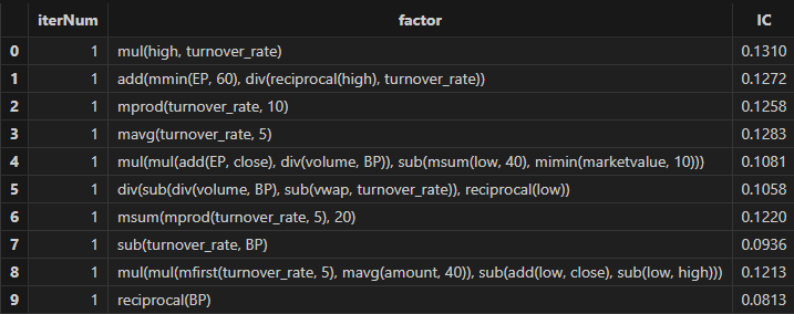
allData = processData() // All data
timer res = trainModel(allData, outerIterNum, innerIterNum, returnNum, icThreshold, corrThreshold)After running, factor formulas can be obtained, as shown in the figure below:
4. Performance Test
To further demonstrate the powerful performance of Shark GPLearn, this section presents a performance comparison between Shark GPLearn, Python GPLearn, and Python Deap under the same testing environment and conditions.
4.1 Test Conditions Setup
Given that Shark GPLearn has a wide range of parameters, this section only sets the shared parameters for Shark GPLearn, Python GPLearn, and Python Deap.
| Training Parameters | Shark GPLearn | Python GPLearn | Deap | Parameter Values |
|---|---|---|---|---|
| Objective Function | fitnessFunc=”pearson” | metric=fitness.make_fitness(…) | toolbox.register(“evaluate”, …) | Custom fitness function |
| Number of Generations | generations | generations | ngen | 5 |
| Population Size | populationSize | population_size | population | 1000 |
| Tournament Size | tournamentSize | tournament_size | tournsize | 20 |
| Constant Term | constRange=0 | const_range=None | addTerminal is not set | As described above |
| Parsimony Coefficient | parsimonyCoefficient | parsimony_coefficient | None | 0.05 |
| Crossover Mutation Probability | crossoverMutationProb | p_crossover | None | 0.6 |
| Subtree Mutation Probability | subtreeMutationProb | p_subtree_mutation | None | 0.01 |
| Hoist Mutation Probability | hoistMutationProb | p_hoist_mutation | None | 0.01 |
| Point Mutation Probability | pointMutationProb | p_point_mutation | None | 0.01 |
| Initialization Method | initMethod=”half” | init_method=”half and half ” | gp.genHalfAndHalf | As described above |
| Initial Tree Depth |
initDepth=[2, 4] restrictDepth=false |
init_depth=(2, 4) |
min_=2 max_=4 |
As described above |
| Parallelism | None | njobs=8(Exclusive) | None | As described above |
The following features are used as training features, and the training target column is ret20 (the future 20-day return of the asset):
| Training Feature | Meaning | Training Feature | Meaning |
|---|---|---|---|
| preclose | Previous close | pctchg | Change in closing price |
| open | Opening price | vwap | Average price |
| close | Closing price | marketvalue | Total market value |
| high | Highest price | turnover_rate | Turnover rate |
| low | Lowest price | EP | Reciprocal of P/E ratio |
| volume | Trading volume | BP | Reciprocal of P/B ratio |
| amount | Trading value |
For the custom fitness function, the Pearson correlation coefficient between factor values and ret20 is used consistently.
For the data and operator settings, the training set includes all trading days from August 12, 2020 to December 31, 2022, and the test set includes all trading days from January 1, 2023 to June 19, 2023. The assets include 3,002 stocks, with the training set containing 1,744,162 records and the test set containing 333,222 records.
4.2 Test Results
| Software | Version | Training Time (s) |
|---|---|---|
| DolphinDB Shark | 3.00.4 2025.09.05 LINUX_ABI x86_64 | 6.3 |
| Python GPLearn | 3.12.7 | 189 |
| Python Deap | 3.12.7 | 1,102 |
The test results show that Shark performs 30.0 times and 174.9 times faster than Python GPLearn and Python DEAP, respectively.
In terms of functionality, Shark offers more features compared to Python GPLearn and Python Deap, such as:
-
Setting
restrictDepth=trueto fully limit the depth of formula trees. -
Using
groupColto enable group-wise operations in the fitness function. -
Setting
windowRangeto specify the range of window functions. -
A richer operator set
functionSetfor enhanced computation support. -
A more convenient expression string parsing and calling method:
sqlColAlias+parseExprfunction.
4.3 Test Environment Configuration
Install DolphinDB Server and configure it in cluster mode. The hardware and software environments involved in this test are as follows:
-
Hardware Environment
Hardware Configuration Kernel 3.10.0-1160.88.1.el7.x86_64 CPU Intel(R) Xeon(R) Gold 5220R CPU @ 2.20GHz GPU NVIDIA A30 24GB(1 unit) Memory 512GB -
Software Environment
Software Version and Configuration Operating System CentOS Linux 7 (Core) DolphinDB Server version: 3.00.4 2025.09.05 LINUX_ABI x86_64 license limit: 16 cores, 128 GB memory
5. FAQ
-
What methods are commonly used in single factor testing?
Single factor testing methods can be divided into three types: ICIR method, regression method, and stratified backtest method. In this tutorial, we mainly used the ICIR method and stratified backtest method for single factor testing.
If the factor expression generated by the genetic algorithm meets the following conditions, it indicates that the factor has strong linear return prediction ability:
-
The RankIC values in both the training and testing periods have the same symbol (positive or negative) and their absolute values exceed the threshold.
-
Stratified backtest returns: Top group > Middle group > Bottom group, and the RankIC remains positive.
-
Stratified backtest returns: Top group < Middle group < Bottom group, and the RankIC remains negative.
If the factor expression generated by the genetic algorithm meets the following condition, it indicates that the factor has non-linear return prediction ability:
-
The stratified backtest results show that the Middle group returns are significantly higher than both the Top and Bottom groups.
-
-
How do I modify relevant configurations in automated factor discovery and customize the logic for factor selection and elimination?
To modify the configuration of automated factor discovery, open the Example_Automated Factor Discovery.dos file and adjust the following parameters:
-
outerIterNum (number of generations for resetting the population)
-
innerIterNum (number of generations for the genetic algorithm)
-
icThreshold (factor expression fitness threshold)
-
corrThreshold (threshold for the mean cross-sectional correlation coefficient with existing factors in the pool)
-
6. Summary
This tutorial fully implements four factor discovery scenarios—daily, minute-level, downsampled, and automated—using the GPLearn genetic algorithm factor discovery functionality of DolphinDB's CPU–GPU heterogeneous computing platform, Shark. Shark GPLearn leverages the powerful computing performance and flexible data processing capabilities of DolphinDB, enabling users to discover more and better-quality factor expressions efficiently.
In the future, Shark GPLearn will further expand support for DolphinDB's built-in functions and allow users to define more flexible custom functions through scripting languages, better meeting the needs of different application scenarios.
Appendix
-
Shark version: 3.00.4 2025.09.09 LINUX_ABI x86_64
-
Code files:
-
Chapter 2:
-
Chapter 3:
-
Chapter 4:
-
-
Masked data files: