Calculating ETF Option Implied Volatility and Greeks
Implied volatility (IV) is a key metric reflecting market expectations of future volatility. It is typically calculated using iterative numerical methods such as the Newton-Raphson or bisection method. These methods, which rely on non-vectorized, loop-based algorithms, can introduce performance bottlenecks in option pricing workflows.
DolphinDB scripts, although written in a scripting language, execute core computations in C++ through an interpreter layer. To optimize performance, DolphinDB introduced Just-In-Time (JIT) compilation, which enhances execution efficiency in scenarios where vectorization is impractical.
This tutorial demonstrates how DolphinDB accelerates the calculation of ETF option implied volatility and Greeks using JIT acceleration. Performance tests show that the DolphinDB script runs at approximately 1.5× the time of a native C++ implementation, achieveing a practical balance between development flexibility and computational performance.
1. Data Structure
1.1 Options Data
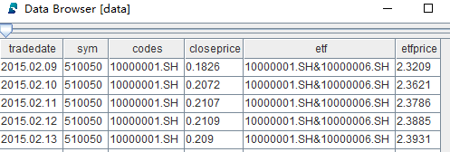
This dataset contains the daily closing prices for ETF options and their underlying ETFs.
| Field | Data Type |
|---|---|
| tradedate | DATE |
| sym | SYMBOL |
| codes | SYMBOL |
| closeprice | DOUBLE |
| etf | SYMBOL |
| etfprice | DOUBLE |
Storage
Partition the data by year:
login("admin", "123456")
dbName = "dfs://optionPrice"
tbName = "optionPrice"
if(existsDatabase(dbName)){
	dropDatabase(dbName)
}
db = database(dbName, RANGE, date(datetimeAdd(2000.01M,0..50*12,'M')))
colNames = `tradedate`sym`codes`closeprice`etf`etfprice
colTypes = [DATE, SYMBOL, SYMBOL, DOUBLE, SYMBOL, DOUBLE]
schemaTable = table(1:0, colNames, colTypes)
db.createPartitionedTable(table=schemaTable, tableName=tbName, partitionColumns=`tradedate)
Query Example
data = select * from loadTable("dfs://optionPrice", "optionPrice") where sym=`510050Where the data is a table variable, containing data as follows:
Use the panel function to pivot the table (in narrow format)
into a closing price matrix:
closPriceWideMatrix = panel(data.codes, data.tradeDate, data.closePrice)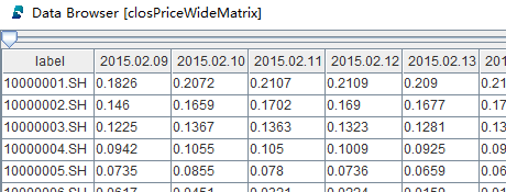
Use the panel function to pivot the table (in narrow format)
into a wide-format price matrix:
etfPriceWideMatrix = panel(data.codes, data.tradeDate, data.etfprice)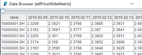
1.2 Options Reference Data
This dataset contains the contract metadata for ETF options.
| Field | Data Type |
|---|---|
| code | STRING |
| name | STRING |
| exemode | INT |
| exeprice | DOUBLE |
| startdate | DATE |
| lastdate | DATE |
| sym | SYMBOL |
| exeratio | DOUBLE |
| exeprice2 | DOUBLE |
| dividenddate | DATE |
| tradecode | STRING |
Storage
Partition the reference data by symbol:
login("admin", "123456")
dbName = "dfs://optionInfo"
tbName = "optionInfo"
if(existsDatabase(dbName)){
	dropDatabase(dbName)
}
db = database(dbName, VALUE, `510050`510300)
colNames = `code`name`exemode`exeprice`startdate`lastdate`sym`exeratio`exeprice2`dividenddate`tradecode
colTypes = [STRING, STRING, INT, DOUBLE, DATE, DATE, SYMBOL, DOUBLE, DOUBLE, DATE, STRING]
schemaTable = table(1:0, colNames, colTypes)
db.createPartitionedTable(table=schemaTable, tableName=tbName, partitionColumns=`sym)
Query Example
contractInfo = select * from loadTable("dfs://optionInfo", "optionInfo") where sym =`5100501.3 Trading Calendars
Trading calendars are stored in single-column CSV files, which can be loaded
using the loadText function.
// File path to the trading calendar
tradingDatesAbsoluteFilename = "/hdd/hdd9/tutorials/jitAccelerated/tradedate.csv"
startDate = 2015.02.01
endDate = 2022.03.01
// Load trading dates from file
allTradingDates = loadText(tradingDatesAbsoluteFilename)
// Generate a vector of trading dates
tradingDates = exec tradedate from allTradingDates where tradedate<endDate and tradedate >startDate
The allTradingDates variable is a single-column table, which is converted into a
vector using the exec statement.
2. Function Implementation
2.1 Implied Volatility
The DolphinDB scripting language requires interpretation before execution. For computation-intensive code that cannot be vectorized, using while/for loops and conditional branches at the script level can be time-consuming. The process of calculating implied volatility, which employs a binary search method with upper/lower bounds for iterative approximation, is ideal for JIT acceleration. Below is the JIT-accelerated binary search implementation for IV:
@jit
def calculateD1JIT(etfTodayPrice, KPrice, r, dayRatio, HLMean){
    skRatio = etfTodayPrice / KPrice
    denominator = HLMean * sqrt(dayRatio)
    result = (log(skRatio) + (r + 0.5 * HLMean * HLMean) * dayRatio) \ denominator
    return result
}

@jit
def calculatePriceJIT(etfTodayPrice, KPrice , r , dayRatio , HLMean , CPMode){
    testResult = 0.0
    if (HLMean <= 0){
        testResult = CPMode * (etfTodayPrice - KPrice)
        return max(testResult, 0.0)
    }else{
        d1 = calculateD1JIT(etfTodayPrice, KPrice, r, dayRatio, HLMean)
        d2 = d1 - HLMean * sqrt(dayRatio)
        price = CPMode * (etfTodayPrice * cdfNormal(0, 1, CPMode * d1) - KPrice * cdfNormal(0, 1, CPMode * d2) * exp(-r * dayRatio))
        return price
    }
}

@jit
def calculateImpvJIT(optionTodayClose, etfTodayPrice, KPrice, r, dayRatio, CPMode){
    v = 0.0
    high = 2.0
    low = 0.0
    do{
        if ((high - low) <= 0.00001){   break   }
        HLMean = (high + low) / 2.0
        if (calculatePriceJIT(etfTodayPrice, KPrice, r, dayRatio, HLMean, CPMode) > optionTodayClose){
            high = HLMean
        } else{
            low = HLMean
        }
    }while(true)
    v = (high + low) / 2.0
    return v
}

def calculateImpv(optionTodayClose, etfTodayPrice, KPrice, r, dayRatio, CPMode){
	originalShape = optionTodayClose.shape()
	optionTodayClose_vec = optionTodayClose.reshape()
	etfTodayPrice_vec = etfTodayPrice.reshape()
	KPrice_vec = KPrice.reshape()
	dayRatio_vec = dayRatio.reshape()
	CPMode_vec = CPMode.reshape()
	impvTmp = each(calculateImpvJIT, optionTodayClose_vec, etfTodayPrice_vec, KPrice_vec, r, dayRatio_vec, CPMode_vec)
	impv = impvTmp.reshape(originalShape)
	return impv
}
The core function for calculating implied volatility is
calculateImpvJIT. Its input parameters
optionTodayClose, etfTodayPrice, KPrice, r,
dayRatio, CPMode are all scalar objects. The
calculatePriceJIT and calculateD1JIT
functions it calls are both encapsulated as JIT functions via the
@jit decorator to accelerate computation.
The calculateImpv function is the final calling function for
implied volatility calculation. Its input parameters optionTodayClose,
etfTodayPrice, KPrice, dayRatio, CPMode are all
matrix objects. Its primary purpose is to transform inputs and outputs to adapt
to argument structure requirements. These input matrices are also used in
subsequent Greeks calculations, such as delta, gamma, vega, and theta. The
following example uses the data of an ETF on February 16, 2015 for IV
calculation.
optionTodayClose

etfTodayPrice

KPrice

dayRatio

CPMode

2.2 Greeks
Greeks (delta, gamma, vega, theta) measure the sensitivity of option prices to various factors. Most Greeks can be vectorized, so JIT is not needed for their calculations.
delta
Delta represents the rate of change of the option price relative to the underlying asset price, i.e., the change in option price per unit change in the underlying asset price. The implementation code is as follows:
def calculateD1(etfTodayPrice, KPrice, r, dayRatio, HLMean){
	skRatio = etfTodayPrice / KPrice
	denominator = HLMean * sqrt(dayRatio)
	result = (log(skRatio) + (r + 0.5 * pow(HLMean, 2)) * dayRatio) / denominator
	return result
}

def cdfNormalMatrix(mean, stdev, X){
	originalShape = X.shape()
	X_vec = X.reshape()
	result = cdfNormal(mean, stdev, X_vec)
	return result.reshape(originalShape)
}

def calculateDelta(etfTodayPrice, KPrice, r, dayRatio, impvMatrix, CPMode){
    delta = iif( impvMatrix <= 0, 0, CPMode *cdfNormal(0, 1, CPMode * calculateD1JIT(etfTodayPrice, KPrice, r, dayRatio, impvMatrix)))
    return delta
}
calculateDelta is the final calling function for delta
calculation. Its input parameters etfTodayPrice, KPrice,
dayRatio, impvMatrix, CPMode are all matrix
objects.
gamma
Gamma represents the rate of change of delta relative to the underlying asset price, i.e., the change in delta value per unit change in the underlying asset price. The implementation code is as follows:
def normpdf(x){
    return exp(-(x*x)/2.0)/sqrt(2*pi)
}

def calculateD1(etfTodayPrice, KPrice, r, dayRatio, HLMean){
	skRatio = etfTodayPrice / KPrice
	denominator = HLMean * sqrt(dayRatio)
	result = (log(skRatio) + (r + 0.5 * pow(HLMean, 2)) * dayRatio) / denominator
	return result
}

def calculateGamma(etfTodayPrice, KPrice, r, dayRatio, impvMatrix){
    gamma = iif(impvMatrix <= 0, 0, (normpdf(calculateD1JIT(etfTodayPrice,  KPrice, r, dayRatio, impvMatrix)) \ (etfTodayPrice * impvMatrix * sqrt(dayRatio))))
    return gamma
}
calculateGamma is the final calling function for gamma
calculation. Its input parameters etfTodayPrice, KPrice,
dayRatio, impvMatrix are all matrix objects.
vega
Vega represents the change in option price per unit change in volatility. The implementation code is as follows:
def normpdf(x){
	return exp(-pow(x, 2)/2.0)/sqrt(2*pi)
}

def calculateD1(etfTodayPrice, KPrice, r, dayRatio, HLMean){
	skRatio = etfTodayPrice / KPrice
	denominator = HLMean * sqrt(dayRatio)
	result = (log(skRatio) + (r + 0.5 * pow(HLMean, 2)) * dayRatio) / denominator
	return result
}

def calculateVega(etfTodayPrice, KPrice, r, dayRatio, impvMatrix){
    vega = iif(impvMatrix <= 0, 0, etfTodayPrice * normpdf(calculateD1JIT(etfTodayPrice, KPrice, r, dayRatio, impvMatrix)) * sqrt(dayRatio))
    return vega\100.0
}
calculateVega is the final calling function for vega
calculation. Its input parameters etfTodayPrice, KPrice,
dayRatio, impvMatrix are all matrix objects.
theta
Theta represents the change in option price due to time decay, i.e., the change in option price per day reduction. The implementation code is as follows:
def calculateD1(etfTodayPrice, KPrice, r, dayRatio, HLMean){
	skRatio = etfTodayPrice / KPrice
	denominator = HLMean * sqrt(dayRatio)
	result = (log(skRatio) + (r + 0.5 * pow(HLMean, 2)) * dayRatio) / denominator
	return result
}

def normpdf(x){
	return exp(-pow(x, 2)/2.0)/sqrt(2*pi)
}

def cdfNormalMatrix(mean, stdev, X){
	originalShape = X.shape()
	X_vec = X.reshape()
	result = cdfNormal(mean, stdev, X_vec)
	return result.reshape(originalShape)
}


def calculateTheta(etfTodayPrice, KPrice, r, dayRatio, impvMatrix, CPMode){
	annualDays = 365
	d1 = calculateD1(etfTodayPrice, KPrice, r, dayRatio, impvMatrix)
	d2 = d1 - impvMatrix * sqrt(dayRatio)
	theta = (-etfTodayPrice * normpdf(d1) * impvMatrix \ (2 * sqrt(dayRatio)) - CPMode * r * KPrice * exp(-r * dayRatio) *cdfNormalMatrix(0, 1, CPMode * d2)) \ annualDays
	result = iif(impvMatrix<= 0, 0, theta)
	return result
}
calculateTheta is the final calling function for theta
calculation. Its input parameters etfTodayPrice, KPrice,
dayRatio, impvMatrix, CPMode are all matrix
objects.
2.3 Single-Day Calculation
Once the core functions are implemented, we can define a function to calculate implied volatility and Greeks for a single day:
def calculateOneDayGreek(closPriceWideMatrix, etfPriceWideMatrix, contractInfo, targetDate){
targetDate_vec = [targetDate]
r = 0
optionTodayClose = getTargetDayOptionClose(closPriceWideMatrix, targetDate_vec)
validContractsToday = optionTodayClose.columnNames()
etfTodayPrice = getTargetDayEtfPrice(etfPriceWideMatrix, targetDate_vec)
KPrice, dayRatio, CPMode = getTargetDayContractInfo(contractInfo, validContractsToday, targetDate_vec)
impvMatrix = calculateImpv(optionTodayClose, etfTodayPrice, KPrice, r, dayRatio, CPMode)
deltaMatrix = calculateDelta(etfTodayPrice, KPrice, r, dayRatio, impvMatrix, CPMode)\(etfTodayPrice*0.01)
gammaMatrix = calculateGamma(etfTodayPrice, KPrice, r, dayRatio, impvMatrix)\(pow(etfTodayPrice, 2) * 0.0001)
vegaMatrix = calculateVega(etfTodayPrice, KPrice, r, dayRatio, impvMatrix)
thetaMatrix = calculateTheta(etfTodayPrice, KPrice, r, dayRatio, impvMatrix, CPMode)
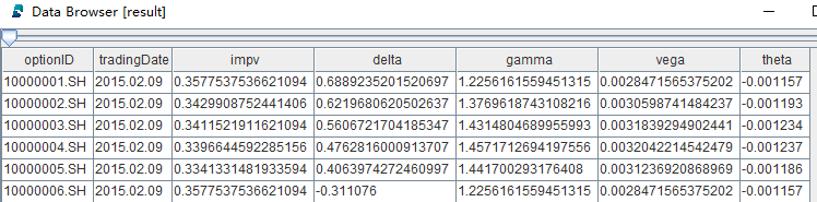
todayTable = table(validContractsToday as optionID, impvMatrix.reshape() as impv, deltaMatrix.reshape() as delta, gammaMatrix.reshape() as gamma, vegaMatrix.reshape() as vega, thetaMatrix.reshape() as theta)
todayTable["tradingDate"] = targetDate
todayTable.reorderColumns!(["optionID", "tradingDate"])
return todayTable
}The input parameters closPriceWideMatrix and etfPriceWideMatrix for
calculateOneDayGreek are matrix objects,
contractInfo is a table object, and targetDate is a scalar
object.
The calculateOneDayGreek function also calls
getTargetDayOptionClose,
getTargetDayEtfPrice, and
getTargetDayContractInfo functions to retrieve valid
information for the calculation date from the full dataset. The code is as
follows:
// Find corresponding prices in the option daily closing price matrix by contract and trading date
def getTargetDayOptionClose(closPriceWideMatrix, targetDate){
	colNum = closPriceWideMatrix.colNames().find(targetDate)
	return closPriceWideMatrix[colNum].transpose().dropna(byRow = false)
}

// Find corresponding prices in the option synthetic futures price matrix by contract and trading date
def getTargetDayEtfPrice(etfPriceWideMatrix, targetDate){
	colNum = etfPriceWideMatrix.colNames().find(targetDate)
	return etfPriceWideMatrix[colNum].transpose().dropna(byRow = false)
}

// Find KPrice, dayRatio, CPMode in the option information table by contract and trading date
def getTargetDayContractInfo(contractInfo, validContractsToday, targetDate){
	targetContractInfo = select code, exemode, exeprice, lastdate, exeprice2, dividenddate, targetDate[0] as tradingDate from contractInfo where Code in validContractsToday
	KPrice = exec iif(tradingDate<dividenddate, exeprice2, exeprice) from targetContractInfo pivot by tradingDate, code
	dayRatio = exec (lastdate-tradingDate)\365.0 from targetContractInfo pivot by tradingDate, Code
	CPMode = exec exemode from targetContractInfo pivot by tradingDate, Code
	return KPrice, dayRatio, CPMode
}
The calculation logic of dayRatio is to divide the remaining holding
period by 365. The specific usage of the calculateOneDayGreek
function will be explained in the next chapter.
2.4 Multi-Day Parallel Calculation
To calculate for multiple days, we can define a parallelized function using
DolphinDB's ploop for parallel execution:
def calculateAll(closPriceWideMatrix, etfPriceWideMatrix, contractInfo, tradingDates, mutable result){
	calculator = partial(calculateOneDayGreek, closPriceWideMatrix, etfPriceWideMatrix, contractInfo)
	timer{
		allResult = ploop(calculator, tradingDates)
	}
	for(oneDayResult in allResult){
		append!(result, oneDayResult)
	}
}
calculateAll is the multi-day parallel calculation function,
primarily utilizing DolphinDB's partial application and ploop
parallel computation. It directly passes the function and parameters to be
parallelized without requiring thread/process pool definitions like other
languages. The specific usage of calculateAll will be explained
in the next chapter.
3. Performance Test
3.1 Test Environment
- CPU: Intel(R) Xeon(R) Silver 4216 CPU @ 2.10GHz
- Logical CPU Cores: 8
- Memory: 64 GB
- OS: 64-bit CentOS Linux 7 (Core)
- DolphinDB Server: 2.00.8 JIT
3.2 Single-Day Calculation
// Define single-day performance test function
def testOneDayPerformance(closPriceWideMatrix, etfPriceWideMatrix, contractInfo, targetDate){
targetDate_vec = [targetDate]
r = 0
optionTodayClose = getTargetDayOptionClose(closPriceWideMatrix, targetDate_vec)
validContractsToday = optionTodayClose.columnNames()
etfTodayPrice = getTargetDayEtfPrice(etfPriceWideMatrix, targetDate_vec)
KPrice, dayRatio, CPMode = getTargetDayContractInfo(contractInfo, validContractsToday, targetDate_vec)
timer{
impvMatrix = calculateImpv(optionTodayClose, etfTodayPrice, KPrice, r, dayRatio, CPMode)
deltaMatrix = calculateDelta(etfTodayPrice, KPrice, r, dayRatio, impvMatrix, CPMode)\(etfTodayPrice*0.01)
gammaMatrix = calculateGamma(etfTodayPrice, KPrice, r, dayRatio, impvMatrix)\(pow(etfTodayPrice, 2) * 0.0001)
vegaMatrix = calculateVega(etfTodayPrice, KPrice, r, dayRatio, impvMatrix)
thetaMatrix = calculateTheta(etfTodayPrice, KPrice, r, dayRatio, impvMatrix, CPMode)
}
todayTable = table(validContractsToday as optionID, impvMatrix.reshape() as impv, deltaMatrix.reshape() as delta, gammaMatrix.reshape() as gamma, vegaMatrix.reshape() as vega, thetaMatrix.reshape() as theta)
todayTable["tradingDate"] = targetDate
todayTable.reorderColumns!(["optionID", "tradingDate"])
return todayTable
}
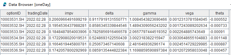
// Execute single-day performance test
oneDay = testOneDayPerformance(closPriceWideMatrix, etfPriceWideMatrix, contractInfo, 2022.02.28)This test runs on data of February 28, 2022, and the option involves 136 contracts. The total execution time is:
- DolphinDB Script: 2.1 ms
- C++ Code: 1.02 ms
3.3 Multi-Day Calculation
The following code tests the performance of multi-day parallel calculations:
// Create a result table
result = table(
array(SYMBOL, 0) as optionID,
array(DATE, 0) as tradingDate,
array(DOUBLE, 0) as impv,
array(DOUBLE, 0) as delta,
array(DOUBLE, 0) as gamma,
array(DOUBLE, 0) as vega,
array(DOUBLE, 0) as theta
)
// Execute multi-day parallel calculation
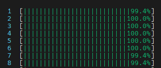
calculateAll(closPriceWideMatrix, etfPriceWideMatrix, contractInfo, tradingDates, result)This test runs on data February 2015 to March 2022, covering 1,729 trading days, and the option involves 3,12 contracts. All the 8 CPU cores are fully utilized.
The total execution time is:
- DolphinDB Script: 300 ms
- C++ Code: 200 ms
CPU utilization during calculation:
4. Conclusion
This tutorial demonstrates how JIT compilation accelerates the calculation of implied volatility and Greeks in ETF options. By leveraging DolphinDB's JIT functionality, implied volatility calculations were significantly sped up, and vectorized operations handled Greeks efficiently. Under full load on 8 CPUs, the DolphinDB script took 300 ms to complete the calculations, while the native C++ code took 200 ms, resulting in a performance difference of approximately 50%. The performance difference between DolphinDB and C++ is minimal for large-scale calculations, making DolphinDB a powerful tool for financial data analysis.
For more detailed features of DolphinDB JIT, please refer to the DolphinDB Tutorial: Just-in-time (JIT) Compilation.