Best Practices for Factor Computation
Factor discovery is the foundation of quantitative trading. Quantitative trading teams must efficiently extract valuable factors from mid- and high-frequency data analysis. Quantitative finance is highly competitive, and factor lifespan shortens as competition grows. Trading teams must use efficient tools and workflows to quickly identify effective factors.
1. Overview
Trading teams commonly use several major technology stacks for factor discovery:
- Data analysis tools like Python and MATLAB
- Third-party factor discovery tools with graphical interfaces
- Custom factor discovery tools built with languages like Java and C++
- Further development on specialized platforms like DolphinDB
Regardless of the technology stack used, the following challenges must be addressed:
- Handling datasets of varying frequencies and scales
- Managing the increasing number of factors
- Efficiently storing and retrieving raw and factor data
- Computing factors of different styles
- Improving development efficiency for factor discovery
- Enhancing factor computation performance (high throughput, low latency)
- Transitioning research factors into production (live trading)
- Addressing engineering challenges for multiple traders or teams, such as code management, unit testing, access control, and large-scale computing
DolphinDB is a high-performance time-series database that integrates distributed computing, real-time stream processing, and distributed storage, making it ideal for factor storage, computation, modeling, backtesting, and live trading. It supports both standalone and cluster deployments, efficiently handling large-scale data from daily to tick-level granularity. Its multi-paradigm programming, extensive function library, and optimized window functions enhance factor development and computation efficiency. With built-in data replay and streaming engines, it enables seamless integration between research and production, while its distributed architecture ensures reliability and scalability.
This article demonstrates DolphinDB's factor computation and storage planning using stock data across various frequencies. Through practical exercises in batch factor computation, real-time factor computation, multi-factor modeling, factor storage planning, and engineering optimization, it presents best practices for factor computation in DolphinDB.
2. Dataset
This article conducts factor analysis based on three types of market datasets: tick-by-tick data, market snapshot, and OHLC data (1-minute and daily). Market snapshot is stored in two formats:
- Each level of market depth is stored as a separate column
- All market depth levels are stored in a single column using an array vector
| Dataset | Database Path | Table Name | Partitioning Scheme |
|---|---|---|---|
| Tick | dfs://tick_SH_L2_TSDB | tick_SH_L2_TSDB | VALUE: day, HASH: [SYMBOL, 20] |
| Snapshot | dfs://snapshot_SH_L2_TSDB | snapshot_SH_L2_TSDB | VALUE: Day, HASH: [SYMBOL, 20] |
| Snapshot (vector storage) | dfs://LEVEL2_Snapshot_ArrayVector | Snap | VALUE: Day, HASH: [SYMBOL, 20] |
| 1-minute OHLC | dfs://k_minute_level | k_minute | VALUE: Month, HASH: [SYMBOL, 3] |
| Daily OHLC | dfs://k_day_level | k_day | VALUE: Year |
2.1. Tick-by-Tick Data
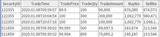
Tick-by-tick data records every individual trade published by the exchange, detailing both the buyer and seller. It is released every 3 seconds, covering all transactions within that period. Each matched trade involves a specific order from both the buyer and the seller.
In the sample dataset above, the fields BuyNo and SellNo indicate the order numbers of the buyer and seller, respectively. Other key fields include:
- SecurityID (Instrument code)
- TradeTime (Transaction timestamp)
- TradePrice (Transaction price)
- TradeQty (Transaction volume)
- TradeAmount (Transaction value)
The tick-by-tick data volume per trading day is approximately 8 GB. The database and table are created based on the partitioning scheme outlined in the table above. Click to view the corresponding script: appendix_2.1_createTickDbAndTable_main.dos.
2.2. Market Snapshot

The market snapshot is published every 3 seconds, including the following fields (at the end of each 3-second interval):
- Intraday cumulative volume (TotalVolumeTrade) and cumulative value (TotalValueTrade) up to that moment.
- Order book snapshot: covering bid and ask orders (Bid for buyers; sellers may be labeled as Offer or Ask), bid/ask prices (BidPrice, OfferPrice), total order quantity (OrderQty), and the number of orders (Orders).
- Latest transaction price (LastPx), opening price (OpenPx), intraday high (HighPx), and intraday low (LowPx).
- Other fields are consistent with tick-by-tick data; refer to the exchange's data dictionary for details.
DolphinDB 2.0 TSDB storage engine supports array vectors, enabling a single cell to store multiple values as a vector. This article provides a detailed comparison between array vector storage and non-array vector storage. In the example, best 10 bid/ask levels are stored as a vector within a single cell.
Database and table creation scripts for both storage formats are available for reference: appendix_2.2_createSnapshotDbAndTable_main.dos.
The market snapshot volume per trading day is approximately 10 GB. The market snapshot is stored as follows:

2.3. 1-minute OHLC Data
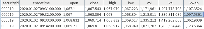
Each stock’s per-minute data includes four price fields: open, high, low, and close prices, along with the trading volume and value for that minute. Additionally, derived indicators such as VWAP can be calculated based on these basic fields. 1-minute OHLC data is aggregated from tick-by-tick trade.
Daily OHLC data follows the same storage format and fields as 1-minute OHLC data and can be aggregated from 1-minute OHLC or high-frequency data.
Database and table creation scripts for OHLC data are available in: appendix_2.3_createTableKMinute_main.dos.
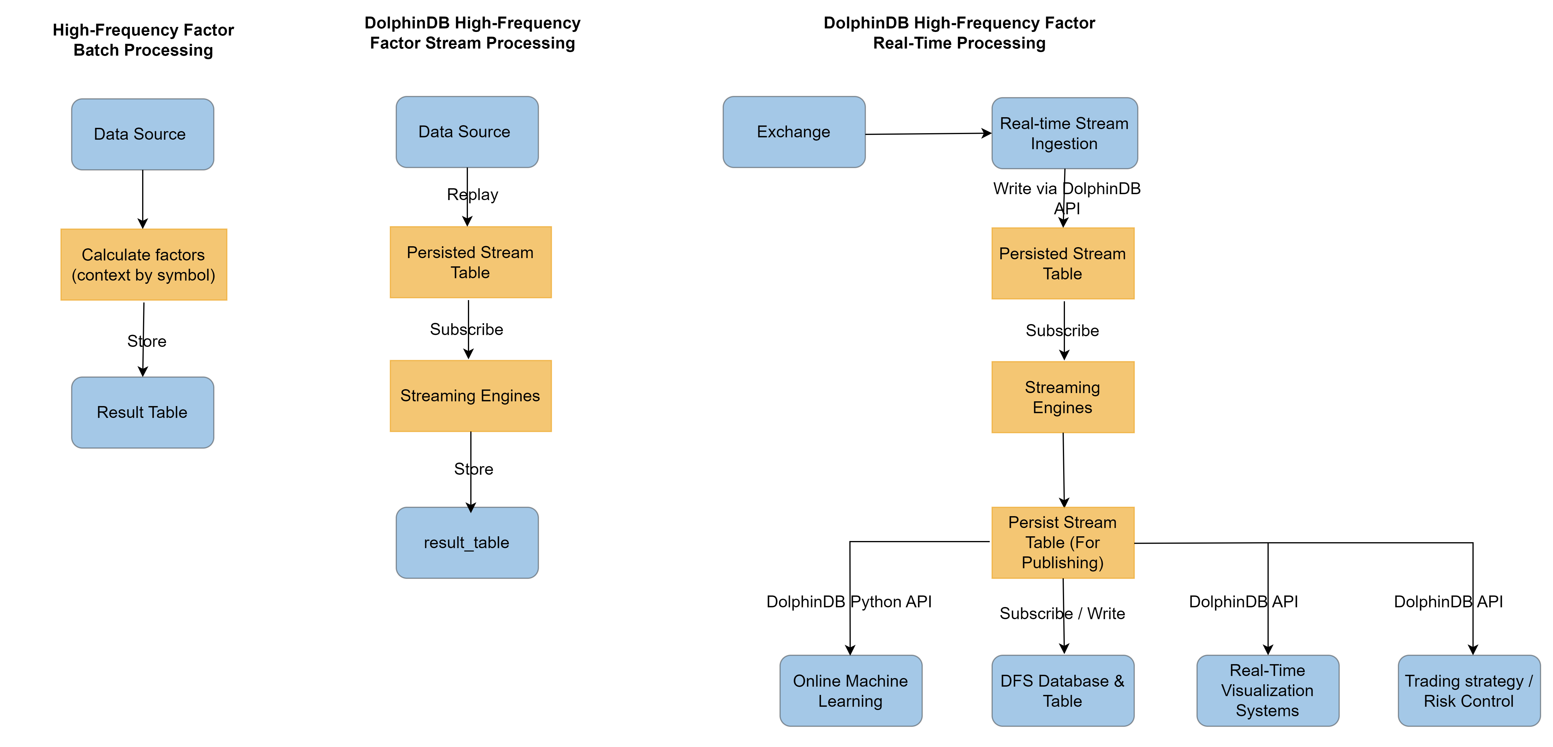
3. Factor Calculation in the Research Environments
During the research environments, factors are typically computed in batches using historical data. DolphinDB offers two calculation modes to meet different factor computation needs:
- Calculation of Panel Data: UDF function parameters are usually vectors, matrices, or tables, with similar output formats.
- Calculation in SQL Queries: UDF function parameters are typically vectors (columns), with output as vectors.
Factor functions should focus solely on the computation logic of a single factor without considering parallel acceleration. The benefits of this approach include:
- Seamless integration of streaming and batch processing
- Easier team collaboration and code management
- A unified framework for running factor computations
3.1. Panel Data Calculation
Panel data uses time as rows, stock ticker as columns, and indicators as values. Performing calculations on panel data can significantly simplify the complexity of scripts (as the calculation expressions can be directly translated from the original mathematical formulas).
Panel data is typically generated using the panel function or
exec combined with pivot by. Each row of
the result represents a timestamp, and each column corresponds to a stock.
                         000001     000002  000003  000004  ...
                        --------- ---------- ------- ------ ---
2020.01.02T09:29:00.000|3066.336 3212.982  257.523 2400.042 ...
2020.01.02T09:30:00.000|3070.247  3217.087 258.696 2402.221 ...
2020.01.02T09:31:00.000|3070.381 3217.170  259.066 2402.029 ...
DolphinDB's row functions and various sliding window functions
can be easily applied to panel data. Factor calculations on panel data simplify
complex logic, allowing execution with just a single line of code. For
example:
- During the calculation of the Alpha 1 factor, the
rowRankfunction is applied for cross-sectional calculations, while theiiffunction can directly filter and compute on vectors. Additionally, sliding window functions likemimaxandmstdperform computations on each column.//alpha 1 //Alpha#001 formula:rank(Ts_ArgMax(SignedPower((returns<0?stddev(returns,20):close), 2), 5))-0.5 @state def alpha1TS(close){ return mimax(pow(iif(ratios(close) - 1 < 0, mstd(ratios(close) - 1, 20),close), 2.0), 5) } def alpha1Panel(close){ return rowRank(X=alpha1TS(close), percent=true) - 0.5 } input = exec close from loadTable("dfs://k_minute","k_minute") where date(tradetime) between 2020.01.01 : 2020.01.31 pivot by tradetime, securityid res = alpha1Panel(input) - When calculating the Alpha 98 factor, three panel datasets—vwap, open, and
vol—are used. Within each matrix, the
rowRankfunction is applied for cross-sectional calculations, while m-functions are used for columnar computations. Additionally, binary operations are performed between matrices. In DolphinDB, all these operations can be accomplished with a single line of code.//alpha 98 //Alpha #98 formula: (rank(decay_linear(correlation(vwap, sum(adv5, 26.4719), 4.58418), 7.18088)) - rank(decay_linear(Ts_Rank(Ts_ArgMin(correlation(rank(open), rank(adv15), 20.8187), 8.62571), 6.95668), 8.07206))) def prepareDataForDDBPanel(raw_data, start_time, end_time){ t = select tradetime,securityid, vwap,vol,open from raw_data where date(tradetime) between start_time : end_time return dict(`vwap`open`vol, panel(t.tradetime, t.securityid, [t.vwap, t.open, t.vol])) } @state def alpha98Panel(vwap, open, vol){ return rowRank(X = mavg(mcorr(vwap, msum(mavg(vol, 5), 26), 5), 1..7),percent=true) - rowRank(X=mavg(mrank(9 - mimin(mcorr(rowRank(X=open,percent=true), rowRank(X=mavg(vol, 15),percent=true), 21), 9), true, 7), 1..8),percent=true) } raw_data = loadTable("dfs://k_minute","k_day") start_time = 2020.01.01 end_time = 2020.12.31 input = prepareDataForDDBPanel(raw_data, start_time, end_time) timer alpha98DDBPanel = alpha98Panel(input.vwap, input.open, input.vol)Factor calculation based on panel data typically involves two stages: panel data preparation and factor computation. The panel data preparation stage can be time-consuming, which impacts overall computational efficiency. To address this, DolphinDB's TSDB engine offers wide format storage, where panel data is directly stored in the database (each column in the panel corresponds to a column in the table). This allows panel data to be accessed directly via SQL queries, eliminating the need for row-column transposition and significantly reducing preparation time. Wide format storage is more efficient than narrow format storage, especially when handling large datasets, and can greatly improve query and computation performance. In Chapter 5, we will provide a detailed comparison of the performance between wide and narrow format storage.
3.2. Calculation in SQL Queries
DolphinDB adopts a columnar structure for both storage and computation. If a factor's calculation only involves a single stock’s time-series data, without cross-sectional analysis across multiple stocks, it can be efficiently performed using SQL queries. This is achieved by grouping data by stock and applying the factor function over a specified time period. When data is partitioned by stock in the database, this method enables highly efficient in-database parallel computation.
def sum_diff(x, y){
    return (x-y)\(x+y)
}

@state
def factorDoubleEMA(price){
    ema_2 = ema(price, 2)
    ema_4 = ema(price, 4)
    sum_diff_1000 = 1000 * sum_diff(ema_2, ema_4)
    return ema(sum_diff_1000, 2) - ema(sum_diff_1000, 3)
}

res = select tradetime, securityid, `doubleEMA as factorname, factorDoubleEMA(close) as val from loadTable("dfs://k_minute","k_minute") where  tradetime between 2020.01.01 : 2020.01.31 context by securityid
In the example above, we define a factor function,
factorDoubleEMA, which operates solely on a stock’s price
series. Using SQL, we apply the context by clause to group data
by stock code and then call the factorDoubleEMA function to
compute the factor series for each stock. Note that context by
is an extension of group by in DolphinDB SQL, making it a
unique feature of DolphinDB. context by is designed for
vectorized computation, where the input and output have the same length.
All technical analysis indicators in TA-Lib are time-series factor functions. These functions can be computed using either SQL queries or the panel data approach. However, factors like Alpha 1 and Alpha 98 (mentioned in Section 2.1) involve both time-series and cross-sectional computations, making them cross-sectional factors. These cannot be encapsulated into a single function and called within a single SQL statement.
For cross-sectional factors, it is recommended to pass the entire table as an input to a UDF factor function, perform SQL operations within the function, and return a table as the output.
//alpha1
def alpha1SQL(t){
	res = select tradetime, securityid, mimax(pow(iif(ratios(close) - 1 < 0, mstd(ratios(close) - 1, 20), close), 2.0), 5) as val from t context by securityid
	return select tradetime, securityid, rank(val, percent=true) - 0.5 as val from res context by tradetime
}
input = select tradetime,securityid, close from loadTable("dfs://k_day_level","k_day") where tradetime between 2010.01.01 : 2010.12.31
alpha1DDBSql = alpha1SQL(input)

//alpha98
def alpha98SQL(mutable t){
	update t set adv5 = mavg(vol, 5), adv15 = mavg(vol, 15) context by securityid
	update t set rank_open = rank(X = open,percent=true), rank_adv15 =rank(X=adv15,percent=true) context by date(tradetime)
	update t set decay7 = mavg(mcorr(vwap, msum(adv5, 26), 5), 1..7), decay8 = mavg(mrank(9 - mimin(mcorr(rank_open, rank_adv15, 21), 9), true, 7), 1..8) context by securityid
	return select tradetime,securityid, `alpha98 as factorname, rank(X =decay7,percent=true)-rank(X =decay8,percent=true) as val from t context by date(tradetime)
}
input = select tradetime,securityid, vwap,vol,open from  loadTable("dfs://k_day_level","k_day") where tradetime between 2010.01.01 : 2010.12.31
alpha98DDBSql = alpha98SQL(input)
3.3. Factor Development at Different Frequencies
Factors derived from data at different frequencies exhibit distinct characteristics. This section illustrates best practices for factor computation based on minute-level, daily, snapshot, and tick-by-tick data.
3.3.1. Minute-Level and Daily Data
Factor computation using daily data often involves complex cross-sectional calculations, which have been demonstrated in the panel data approach. Simpler computations, however, are similar to those used for minute-level factors.
For minute-level data, the following example demonstrates the computation of
intraday return skewness. Since this type of calculation only involves
fields within the table, it is typically performed using the SQL with the
group by statement:
defg dayReturnSkew(close){
	return skew(ratios(close))
}

minReturn = select `dayReturnSkew as factorname, dayReturnSkew(close) as val from loadTable("dfs://k_minute_level", "k_minute") where date(tradetime) between 2020.01.02 : 2020.01.31 group by date(tradetime) as tradetime, securityid

/* output
tradetime  securityid factorname    val
---------- ---------- ------------- -------
2020.01.02 000019     dayReturnSkew 11.8328
2020.01.02 000048     dayReturnSkew 11.0544
2020.01.02 000050     dayReturnSkew 10.6186
*/
3.3.2. Stateful Factor Computation for Market Snapshot
Stateful factors depend on previous results, such as sliding window and aggregation calculations.
In the following example, the UDF function flow takes four
column fields as input. By using the mavg and
iif functions, factor can be computed directly in
SQL:
@state
def flow(buy_vol, sell_vol, askPrice1, bidPrice1){
        buy_vol_ma = round(mavg(buy_vol, 5*60), 5)
        sell_vol_ma = round(mavg(sell_vol, 5*60), 5)
        buy_prop = iif(abs(buy_vol_ma+sell_vol_ma) < 0, 0.5 , buy_vol_ma/ (buy_vol_ma+sell_vol_ma))
        spd = askPrice1 - bidPrice1
        spd = iif(spd < 0, 0, spd)
        spd_ma = round(mavg(spd, 5*60), 5)
        return iif(spd_ma == 0, 0, buy_prop / spd_ma)
}

res_flow = select TradeTime, SecurityID, `flow as factorname, flow(BidOrderQty[1],OfferOrderQty[1], OfferPrice[1], BidPrice[1]) as val from loadTable("dfs://LEVEL2_Snapshot_ArrayVector","Snap") where date(TradeTime) <= 2020.01.30 and date(TradeTime) >= 2020.01.01 context by SecurityID

/* output sample
TradeTime               SecurityID factorname val
----------------------- ---------- ---------- -----------------
2020.01.22T14:46:27.000 110065     flow       3.7587
2020.01.22T14:46:30.000 110065     flow       3.7515
2020.01.22T14:46:33.000 110065     flow       3.7443
...
*/
3.3.3. Stateless Factor Computation for Market Snapshot
Traditionally, Level 2 market snapshot is stored as multiple columns, with matrices used for weighted calculations. A more efficient approach is to store the data as array vectors, allowing function reuse while enhancing efficiency and reducing resource consumption.
The following example calculates the weighted skewness factor for quotes. Using array vector storage reduces computation time from 4 seconds to 2 seconds.
def mathWghtCovar(x, y, w){
 	v = (x - rowWavg(x, w)) * (y - rowWavg(y, w))

	return rowWavg(v, w)
 }

@state
 def mathWghtSkew(x, w){
 	x_var = mathWghtCovar(x, x, w)
 	x_std = sqrt(x_var)
 	x_1 = x - rowWavg(x, w)
	x_2 = x_1*x_1
 	len = size(w)
 	adj = sqrt((len - 1) * len) \ (len - 2)
	skew = rowWsum(x_2, x_1) \ (x_var * x_std) * adj \ len
	return iif(x_std==0, 0, skew)
 }

//weights:
 w = 10 9 8 7 6 5 4 3 2 1

//Weighted skewness factorfactor
resWeight =  select TradeTime, SecurityID, `mathWghtSkew as factorname, mathWghtSkew(BidPrice, w)  as val from loadTable("dfs://LEVEL2_Snapshot_ArrayVector","Snap")  where date(TradeTime) = 2020.01.02 map
resWeight1 =  select TradeTime, SecurityID, `mathWghtSkew as factorname, mathWghtSkew(matrix(BidPrice0,BidPrice1,BidPrice2,BidPrice3,BidPrice4,BidPrice5,BidPrice6,BidPrice7,BidPrice8,BidPrice9), w)  as val from loadTable("dfs://snapshot_SH_L2_TSDB", "snapshot_SH_L2_TSDB")  where date(TradeTime) = 2020.01.02 map


/* output
 TradeTime               SecurityID factorname val
----------------------- ---------- ---------- ------
...
2020.01.02T09:30:09.000 113537     array_1    -0.8828
2020.01.02T09:30:12.000 113537     array_1    0.7371
2020.01.02T09:30:15.000 113537     array_1    0.6041
...
*/
3.3.4. Minute Aggregation Based on Market Snapshot
It is often necessary to aggregate market snapshot into minute-level OHLC (Open, High, Low, Close) data. The following example illustrates a common approach for this scenario:
//Calculate OHLC based on market snapshot, vwap
tick_aggr = select first(LastPx) as open, max(LastPx) as high, min(LastPx) as low, last(LastPx) as close, sum(totalvolumetrade) as vol,sum(lastpx*totalvolumetrade) as val,wavg(lastpx, totalvolumetrade) as vwap from loadTable("dfs://LEVEL2_Snapshot_ArrayVector","Snap") where date(TradeTime) <= 2020.01.30 and date(TradeTime) >= 2020.01.01 group by SecurityID, bar(TradeTime,1m)
3.3.5. Main Buy Volume Proportion Calculation with Tick Data
Tick-by-tick data is typically used for calculations involving fields like
trade volume. The following example calculates the ratio of the main buyer's
trade volume to the total trade volume for each day. It uses the SQL
approach to leverage in-database parallel computation and employs the
csort statement to sort the data within each group by
timestamp:
@state
def buyTradeRatio(buyNo, sellNo, tradeQty){
    return cumsum(iif(buyNo>sellNo, tradeQty, 0))\cumsum(tradeQty)
}

factor = select TradeTime, SecurityID, `buyTradeRatio as factorname, buyTradeRatio(BuyNo, SellNo, TradeQty) as val from loadTable("dfs://tick_SH_L2_TSDB","tick_SH_L2_TSDB") where date(TradeTime)<2020.01.31 and time(TradeTime)>=09:30:00.000 context by SecurityID, date(TradeTime) csort TradeTime

/* output
TradeTime           SecurityID factorname val
------------------- ---------- ---------- ------
2020.01.08T09:30:07 511850     buyTradeRatio    0.0086
2020.01.08T09:30:31 511850     buyTradeRatio    0.0574
2020.01.08T09:30:36 511850     buyTradeRatio    0.0569
...
*/
4. Factor Calculation in Streaming
DolphinDB provides a real-time stream computing framework, allowing factor functions developed during research to be seamlessly deployed in production, enabling unified batch and stream processing. This integration not only enhances development efficiency but also leverages the highly optimized stream computing framework for superior calculation performance.
At the core of DolphinDB’s streaming solution are the streaming engines and stream
tables. The streaming engine supports time-series processing, cross-sectional
analysis, window operations, table joins, and anomaly detection, etc. Stream tables
function like message brokers or topics within a messaging system, allowing data to
be published and subscribed to. Both the streaming engine and stream tables are
DolphinDB tables, meaning data can be injected into them using the
append! function. Since the streaming engine also outputs
tables, multiple streaming engines can be flexibly combined, like building blocks,
to construct streaming processing pipelines.
4.1. Incremental Computing in Stream Processing
In financial applications, both raw data and computed indicators typically
exhibit temporal continuity. For a simple five-period moving average,
mavg(close, 5), each update can be performed incrementally.
When a new data point is received, subtract the value from the fifth prior
period and add the new value to the existing sum. This avoids recalculating the
sum of each update, improving computational efficiency. This approach, known as
incremental computation, is a core concept in stream processing that
significantly reduces real-time computation latency.
DolphinDB provides a wide range of built-in operators optimized for quantitative
finance, many of which leverage incremental computation. Additionally, DolphinDB
implements incremental optimization for user-defined functions. In the previous
section, some UDF factor functions were marked with the @state
modifier, indicating that they support incremental computation.
4.1.1. Active Buy Volume Ratio
The following example demonstrates how to implement the active buy volume ratio factor using the reactive state engine for streaming-based incremental computation.
@state
def buyTradeRatio(buyNo, sellNo, tradeQty){
    return cumsum(iif(buyNo>sellNo, tradeQty, 0))\cumsum(tradeQty)
}

tickStream = table(1:0, `SecurityID`TradeTime`TradePrice`TradeQty`TradeAmount`BuyNo`SellNo, [SYMBOL,DATETIME,DOUBLE,INT,DOUBLE,LONG,LONG])
result = table(1:0, `SecurityID`TradeTime`Factor, [SYMBOL,DATETIME,DOUBLE])
factors = <[TradeTime, buyTradeRatio(BuyNo, SellNo, TradeQty)]>
demoEngine = createReactiveStateEngine(name="demo", metrics=factors, dummyTable=tickStream, outputTable=result, keyColumn="SecurityID")
The above script creates the demo reactive state engine grouping by SecurityID, with input message format matching the in-memory table tickStream. The indicators to be computed are defined in “factors”, including TradeTime (an original field from the input table), and a factor function that needs to be computed. The results are stored in the in-memory table result, which includes the defined factors. Notably, the UDF factor function remains identical to the one used in batch computation.
Once the engine is created, data can be inserted into it, and the results can be observed in real time.
insert into demoEngine values(`000155, 2020.01.01T09:30:00, 30.85, 100, 3085, 4951, 0)
insert into demoEngine values(`000155, 2020.01.01T09:30:01, 30.86, 100, 3086, 4951, 1)
insert into demoEngine values(`000155, 2020.01.01T09:30:02, 30.80, 200, 6160, 5501, 5600)

select * from result
/*
SecurityID TradeTime           Factor
---------- ------------------- ------
000155     2020.01.01T09:30:00 1
000155     2020.01.01T09:30:01 1
000155     2020.01.01T09:30:02 0.5
*/
This case illustrates how DolphinDB simplifies streaming-driven incremental computation. A UDF factor validated in research can be transitioned to production by instantiating a stream processing engine, achieving seamless real-time factor computation with minimal operational overhead.
4.1.2. Large/Small Orders
In real-time processing, large/small order classification serves as a foundational component for tracking institutional vs. retail investor activities. However, real-time implementation faces two key challenges:
- State Dependency: Large/small order determination requires historical state. Without incremental computation, processing afternoon data would require re-scanning all morning order records, introducing unacceptable computational overhead in real-time pipelines.
- Multi-Stage Computation:
- Phase 1: Group orders by ID, classify them as large/small based on cumulative execution volume thresholds.
- Phase 2: Aggregate order classes by ticker to calculate metrics (counts, notional amounts).
Large/small orders are dynamically defined – a "small" order may transition to "large" as its cumulative volume grows. DolphinDB addresses this with two native functions:
dynamicGroupCumsum: Real-time incremental cumulative sum within dynamically evolving groups.dynamicGroupCumcount: Real-time incremental count within evolving groups.
For implementation details, refer to: appendix_4.1.2_streamComputationOfSmallInflowRate_main.dos.
@state
 def factorSmallOrderNetAmountRatio(tradeAmount, sellCumAmount, sellOrderFlag, prevSellCumAmount, prevSellOrderFlag, buyCumAmount, buyOrderFlag, prevBuyCumAmount, prevBuyOrderFlag){

	cumsumTradeAmount = cumsum(tradeAmount)
 	smallSellCumAmount, bigSellCumAmount = dynamicGroupCumsum(sellCumAmount, prevSellCumAmount, sellOrderFlag, prevSellOrderFlag, 2)

	smallBuyCumAmount, bigBuyCumAmount = dynamicGroupCumsum(buyCumAmount, prevBuyCumAmount, buyOrderFlag, prevBuyOrderFlag, 2)

	f = (smallBuyCumAmount - smallSellCumAmount) \ cumsumTradeAmount
	return smallBuyCumAmount, smallSellCumAmount, cumsumTradeAmount, f
}

def createStreamEngine(result){
	tradeSchema = createTradeSchema()
	result1Schema = createResult1Schema()
	result2Schema = createResult2Schema()
	engineNames = ["rse1", "rse2", "res3"]
	cleanStreamEngines(engineNames)

	metrics3 = <[TradeTime, factorSmallOrderNetAmountRatio(tradeAmount, sellCumAmount, sellOrderFlag, prevSellCumAmount, prevSellOrderFlag, buyCumAmount, buyOrderFlag, prevBuyCumAmount, prevBuyOrderFlag)]>
	rse3 = createReactiveStateEngine(name=engineNames[2], metrics=metrics3, dummyTable=result2Schema, outputTable=result, keyColumn="SecurityID")

	metrics2 = <[BuyNo, SecurityID, TradeTime, TradeAmount, BuyCumAmount, PrevBuyCumAmount, BuyOrderFlag, PrevBuyOrderFlag, factorOrderCumAmount(TradeAmount)]>
	rse2 = createReactiveStateEngine(name=engineNames[1], metrics=metrics2, dummyTable=result1Schema, outputTable=rse3, keyColumn="SellNo")

	metrics1 = <[SecurityID, SellNo, TradeTime, TradeAmount, factorOrderCumAmount(TradeAmount)]>
	return createReactiveStateEngine(name=engineNames[0], metrics=metrics1, dummyTable=tradeSchema, outputTable=rse2, keyColumn="BuyNo")
}
The stateful function factorSmallOrderNetAmountRatio
calculates the ratio of small order net flow to total trading volume. This
is implemented through an engine pipeline, which automatically chains three
reactive state engines in the required computational sequence:
- Engine rse3 is grouped by SecurityID and Computes the small order net flow ratio (small order net inflow / total traded notional) within each group.
- In the upstream stages, Engine rse1 is grouped by BuyNo (Bid-side order ID), and Engine rse2 is grouped by SellNo (Ask-side order ID) . These engines track the cumulative execution volume per order to dynamically classify orders as large or small based on adjustable thresholds.
We validate the pipeline using sample tick data to demonstrate the real-time computation process.
result = createResultTable()
rse = createStreamEngine(result)
insert into rse values(`000155, 1000, 1001, 2020.01.01T09:30:00, 20000)
insert into rse values(`000155, 1000, 1002, 2020.01.01T09:30:01, 40000)
insert into rse values(`000155, 1000, 1003, 2020.01.01T09:30:02, 60000)
insert into rse values(`000155, 1004, 1003, 2020.01.01T09:30:03, 30000)

select * from result
/*
SecurityID TradeTime smallBuyOrderAmount smallSellOrderAmount totalOrderAmount factor
---------- ------------------- ------------------- -------------------- ---------------- ------
000155     2020.01.01T09:30:00 20000               20000                20000            0
000155     2020.01.01T09:30:01 60000               60000                60000            0
000155     2020.01.01T09:30:02 0                   120000               120000           -1
000155     2020.01.01T09:30:03 30000               150000               150000           -0.8
*/
4.1.3. Streamlined Implementation of Factor Alpha 1
The previous large/small order example demonstrates how complex factors may require multi-engine pipelines. Manually constructing these pipelines is time-consuming.
For single-grouping cases, DolphinDB provides the
streamEngineParser to automate this process. Here we
implement the Alpha 1 factor using this parser. See full code: appendix_4.1.3_StreamComputationOfAlpha1Factor_main.dos.
@state
def alpha1TS(close){
	return mimax(pow(iif(ratios(close) - 1 < 0, mstd(ratios(close) - 1, 20),close), 2.0), 5)
}

def alpha1Panel(close){
	return rowRank(X=alpha1TS(close), percent=true) - 0.5
}

inputSchema = table(1:0, ["SecurityID","TradeTime","close"], [SYMBOL,TIMESTAMP,DOUBLE])
result = table(10000:0, ["TradeTime","SecurityID", "factor"], [TIMESTAMP,SYMBOL,DOUBLE])
metrics = <[SecurityID, alpha1Panel(close)]>
streamEngine = streamEngineParser(name="alpha1Parser", metrics=metrics, dummyTable=inputSchema, outputTable=result, keyColumn="SecurityID", timeColumn=`tradetime, triggeringPattern='keyCount', triggeringInterval=4000)
The Alpha 1 factor involves both time-series and cross-sectional
computations, requiring a combination of reactive state engines and
cross-sectional engines. However, the above implementation leverages
streamEngineParser to automatically generate all
necessary engines, significantly streamlining the process.
The previous examples illustrate how DolphinDB's streaming engine enables incremental factor calculation while seamlessly integrating research-stage factor logic into production. This addresses the long-standing challenge in quantitative finance of maintaining separate implementations for historical backtesting and real-time execution. With DolphinDB, the entire workflow—from market data ingestion and real-time processing to post-trade analysis—operates within a unified framework, ensuring data consistency and enhancing both research and trading efficiency.
4.2. Factor Computation via Data Replay
The previous section introduced DolphinDB’s unified batch-stream processing, where the same factor function is used for both batch and stream calculation, ensuring code reuse.
DolphinDB also offers a more streamlined approach: during historical data modeling, data replay can be used to compute factors directly with the streaming engine, eliminating the need for a separate batch processing pipeline. This ensures consistency in computation logic while improving development efficiency.
While the previous section demonstrated the computation of
factorDoubleEMA using SQL-based batch processing, this
section illustrates how to calculate factorDoubleEMA via data
replay in a streaming context. For complete implementation details, refer to
appendix_4.2_streamComputationOfDoubleEmaFactor_main.dos.
//Create a streaming engine and pass the factor algorithm factorDoubleEMA

factors = <[TradeTime, factorDoubleEMA(close)]>
 demoEngine = createReactiveStateEngine(name=engineName, metrics=factors, dummyTable=inputDummyTable, outputTable=resultTable, keyColumn="SecurityID")


//demo_engine subscribes to the snapshotStreamTable table

subscribeTable(tableName=snapshotSharedTableName, actionName=actionName, handler=append!{demoEngine}, msgAsTable=true)

//Create a data source for replay; during market hours, switch to writing real-time market data directly to snapshotStreamTable
inputDS = replayDS(<select SecurityID, TradeTime, LastPx from tableHandle where date(TradeTime)<2020.07.01>, `TradeTime, `TradeTime)
4.3. Integration with Trading Systems
DolphinDB provides APIs for a variety of popular programming languages, including C++, Java, JavaScript, C#, Python, and Go. Programs written in these languages can leverage the corresponding DolphinDB APIs to subscribe to streaming tables from a DolphinDB server. Below is a simple example demonstrating how to subscribe to a streaming table using the Python API. For the details, refer to appendix_4.3.1_python_callback_handler_subscribing_stream_main.py.
current_ddb_session.subscribe(host=DDB_datanode_host,tableName=stream_table_shared_name,actionName=action_name,offset=0,resub=False,filter=None,port=DDB_server_port,
handler=python_callback_handler,# Pass the callback function to receive messages.
)
In live trading, streaming data is typically ingested into message queues in real time for downstream consumption. DolphinDB supports pushing results to messaging middleware for integration with trading systems. The example demonstrates how to use DolphinDB’s open-source ZMQ plugin to stream real-time results into a ZMQ message queue, enabling consumption by subscribers such as trading systems or market display modules. Beyond ZMQ, DolphinDB provides support for other mainstream messaging systems. All DolphinDB plugins are open-source, and users can develop custom plugins based on the open-source framework as needed.
An example of pushing streaming data from DolphinDB to a ZMQ message queue:
- Start the ZMQ Message Consumer
This program acts as the ZeroMQ message queue server, listening for incoming data. For the full implementation, refer to appendix_4.3.2_zmq_consuming_ddb_stream_main.py.
zmq_context = Context() zmq_bingding_socket = zmq_context.socket(SUB) # Set socket options zmq_bingding_socket.bind("tcp://*:55556") async def loop_runner(): while True: msg=await zmq_bingding_socket.recv() # Blocking loop until stream data is received print(msg) # Implement downstream message processing logic here asyncio.run(loop_runner()) - Initialize Factor Streaming Computation and Publishing result
Once the ZMQ consumer is running, DolphinDB needs to start stream processing and publish the results. The following code demonstrates the DolphinDB implementation. For details of DolphinDB, refer to appendix_4.3.3_streamComputationOfDoubleEmaFactorPublishingOnZMQ_main.dos.
// Table scheme for message queue output
resultSchema=table(1:0,["SecurityID","TradeTime","factor"], [SYMBOL,TIMESTAMP,DOUBLE])

def zmqPusherTable(zmqSubscriberAddress,schemaTable){
	SignalSender=def (x) {return x}
	pushingSocket = zmq::socket("ZMQ_PUB", SignalSender)
	zmq::connect(pushingSocket, zmqSubscriberAddress)
	pusher = zmq::createPusher(pushingSocket, schemaTable)
	return pusher
}

// demoEngine pushes data to ZMQ queue - modify this string for different ZMQ addresses
zmqSubscriberAddress="tcp://192.168.1.195:55556"

// Create a table to send ZMQ packets to the specified address, with scheme matching resultSchema
pusherTable=zmqPusherTable(zmqSubscriberAddress,resultSchema)

// Create a streaming engine outputting to pusher
demoEngine = createReactiveStateEngine(name="reactiveDemo", metrics=<[TradeTime,doubleEma(LastPx)]>, dummyTable=snapshotSchema, outputTable=pusherTable, keyColumn="SecurityID",keepOrder=true)
5. Factor Storage and Query Optimization
This chapter discusses selecting the most efficient storage model based on usage scenarios, query patterns, and storage strategies. The test environment is as follows:
- Cluster: Single-machine deployment
- Nodes: 3 data nodes (Linux OS)
- Hardware: 16 threads/node, 3 SSDs/node for storage
Factor storage requires careful consideration of three key aspects: the choice of storage engine, the data model, and the partitioning strategy. OLAP engines are best suited for large-scale batch processing and complex aggregation queries, while TSDB engines excel in queries for series with optimized performance and functionality. For the data model, narrow format storage offers high flexibility but comes with increased data redundancy, whereas wide format storage improves efficiency but requires schema changes when adding new factors or stocks. Partitioning can be based on time, stock code, or factor name, with OLAP engines performing best with partitions around 100MB and TSDB engines optimizing query efficiency with partition sizes between 100MB and 1GB.
Using a dataset of 4000 stocks, 1000 factors, and minute-level data, we evaluate three storage strategies:
- OLAP database, narrow format storage:
Each row stores a single factor value for one stock at a given time. Partition data by month (using TradeTime column) and factor name (FactorName).
- TSDB database, narrow format storage:
Each row stores as a single factor value for one stock at a given time. Partition data by month (using TradeTime column) and factor name (FactorName). Within each partition, sort data by security ID (SecurityID) and trade time (TradeTime).
- TSDB database, wide format storage:
Each row stores all stocks for one factor or all factors for one stock. Partition data by month (using TradeTime column) and factor name (FactorName). Within each partition, sort data by factor name (FactorName) and trade time (TradeTime).
Narrow Format Storage:
| tradetime | securityid | factorname | factorval |
|---|---|---|---|
| 2020:12:31 09:30:00 | sz000001 | factor1 | 143.20 |
| 2020:12:31 09:30:00 | sz000001 | factor2 | 142.20 |
| 2020:12:31 09:30:00 | sz000002 | factor1 | 142.20 |
| 2020:12:31 09:30:00 | sz000002 | factor2 | 142.20 |
Wide Format Storage:
| tradetime | factorname | sz000001 | sz000002 | sz000003 | sz000004 | sz000005 | ...... | sz600203 |
|---|---|---|---|---|---|---|---|---|
| 2020:12:31 09:30:00 | factor1 | 143.20 | 143.20 | 143.20 | 143.20 | 143.20 | ....... | 143.20 |
| 2020:12:31 09:30:00 | factor2 | 143.20 | 143.20 | 143.20 | 143.20 | 143.20 | ....... | 143.20 |
5.1. Factor Storage
We evaluate three storage models by storing one year of minute-level data for five factors, comparing their efficiency in terms of data volume, storage usage, and write performance.
| Storage Format | Engine | Total Rows | Bytes per Row | Data Size (GB) | Actual Storage (GB) | Compression Ratio | Write Time (s) | Peak IO (MB/s) |
|---|---|---|---|---|---|---|---|---|
| Narrow Format | OLAP | 1,268,080,000 | 24 | 28.34 | 9.62 | 0.34 | 150 | 430 |
| Narrow Format | TSDB | 1,268,080,000 | 24 | 28.34 | 9.03 | 0.32 | 226 | 430 |
| Wide Format | TSDB | 317,020 | 32,012 | 9.45 | 8.50 | 0.90 | 38 | 430 |
Analysis of Results
- Write Performance: TSDB wide format writes 4× faster than OLAP narrow format and 5× faster than TSDB narrow format.
- Storage Efficiency: OLAP and TSDB narrow format have similar storage sizes, while TSDB wide format is slightly smaller.
- Compression Ratio: TSDB narrow format achieves the highest compression, followed by OLAP narrow format, with TSDB wide format performing the worst.
Key Influencing Factors
- Data Volume & Efficiency: narrow format stores 3× more data per row, making TSDB wide format faster and more space-efficient, though its compression suffers.
- Data Randomness: High randomness in the dataset reduces compression efficiency in TSDB wide format.
- Storage Engine Optimization: TSDB narrow format applies sorting and indexing, slightly impacting its storage, write speed, and compression compared to OLAP.
For detailed implementation, refer to appendix_5.1_factorDataSimulation.zip.
5.2. Factor Query Performance Testing
To evaluate query performance under large-scale data conditions, we simulate a dataset of 4,000 stocks, 200 factors, and one year of minute-level data. The table below summarizes the dataset characteristics and partitioning strategies:
| Storage Format | Engine | Stocks | Factors | Time Span | Granularity | Total Rows | Bytes per Row | Data Size (GB) | Partitioning |
|---|---|---|---|---|---|---|---|---|---|
| Narrow Format | OLAP | 4000 | 200 | 1 year | Minute | 50,723,200,000 | 24 | 1133.75 | VALUE(day) + VALUE(factor) |
| Narrow Format | TSDB | 4000 | 200 | 1 year | Minute | 50,723,200,000 | 24 | 1133.75 | VALUE(month) + VALUE(factor) |
| Wide Format | TSDB | 4000 | 200 | 1 year | Minute | 12,680,800 | 32012 | 340.19 | VALUE(month) + VALUE(factor) |
We evaluate query performance across OLAP narrow format, TSDB narrow format, and TSDB wide format by testing multiple query scenarios. For detailed script, refer to appendix_5.2_factorQueryTest.dos.
| Storage Format | Engine | Rows Retrieved | Bytes per Row | Latency (ms) |
|---|---|---|---|---|
| Narrow Format | OLAP | 1 | 24 | 100 |
| Narrow Format | TSDB | 1 | 24 | 6 |
| Wide Format | TSDB | 1 | 20 | 2 |
- TSDB significantly outperforms OLAP for point querieswithin a given time range.
- Due to fewer rows, TSDB wide format achieves the fastest response time.
Query 2: Single Factor, Single Stock, One Year (Minute-Level Data)
| Storage Format | Engine | Data Size (MB) | Query Time (s) |
|---|---|---|---|
| Narrow Format | OLAP | 1.5 | 0.9 |
| Narrow Format | TSDB | 1.5 | 0.03 |
| Wide Format | TSDB | 1.2 | 0.02 |
- TSDB wide format is the fastest, as it requires fewer file reads due to larger partitions and pre-sorted data.
- OLAP narrow format is the slowest because it scans more partitions.
Query 3: Single Factor, All Stocks, One Year (Minute-Level Data)
| Storage Format | Engine | Data Size (GB) | Query Time (s) |
|---|---|---|---|
| Narrow Format | OLAP | 5.7 | 8.9 |
| Narrow Format | TSDB | 5.7 | 12.4 |
| Wide Format | TSDB | 1.9 | 3.8 |
Query 4: Three Factors, All Stocks, One Year (Minute-Level Data)
| Storage Format | Engine | Data Size (GB) | Query Time (s) |
|---|---|---|---|
| Narrow Format | OLAP | 17.0 | 17.7 |
| Narrow Format | TSDB | 17.0 | 25.9 |
| Wide Format | TSDB | 5.7 | 10.7 |
- Query time scales linearly with data volume.
- TSDB wide format remains the most efficient due to its compact storage.
Query 5: Single Stock, All Factors, One Year (Minute-Level Data)
For wide format storage, queries should only select the necessary stock code column. The SQL query are as follows:
// Query a narrow table, retrieve all fields via wildcard (*)
tsdb_symbol_all=select  * from tsdb_min_factor where symbol=`sz000056

// Query a wide table, selectively retrieve specific fields
select mtime,factorname,sz000001 from tsdb_wide_min_factor
The results show that both TSDB wide format and TSDB narrow format achieve fast query performance, whereas OLAP narrow format takes over 100 times longer. This discrepancy arises because OLAP narrow format partitions data by time and factor, requiring a full table scan to retrieve all factors for a single stock. In contrast, TSDB wide format only needs to read three columns, significantly improving query efficiency.
Furthermore, TSDB narrow format also demonstrates relatively good query performance compared to OLAP narrow format. This is due to TSDB’s built-in indexing on stock codes, enabling fast data retrieval.
In summary, factor storage strategies should be planned based on expected query patterns. Given the performance results, we recommend using TSDB wide format for factor storage to optimize query efficiency.
5.3. Real-Time Panel Data Retrieval
Different storage models allow real-time panel data generation using the following DolphinDB scripts.
Single-Factor, All Stocks, One Year (Minute-Level Panel Data)
// Narrow format storage
olap_factor_year_pivot_1=select val from olap_min_factor where factorcode=`f0002 pivot by tradetime,symbol
// Wide format storage
wide_tsdb_factor_year=select * from tsdb_wide_min_factor where factorname =`f0001| Storage Format | Engine | Data Size (GB) | Query Time (s) |
|---|---|---|---|
| Narrow Format | OLAP | 1.9 | 41.2 |
| Narrow Format | TSDB | 1.9 | 32.9 |
| Wide Format | TSDB | 1.9 | 3.3 |
TSDB wide format achieves over 10× faster query performance than both OLAP and
TSDB narrow format. This advantage stems from its inherent data structure, which
is already stored in a panel-like format, eliminating the need for
transformation. In contrast, both OLAP and TSDB narrow format require a
pivot by operation to reshape the data, introducing
additional deduplication and sorting overhead. As dataset size increases, this
overhead becomes the primary performance bottleneck, further widening the gap
between wide and narrow formats.
Three-Factor, All Stocks, One Year (Minute-Level Panel Data)
// Narrow format storage
olap_factor_year_pivot=select val from olap_min_factor where factorcode in ('f0001','f0002','f0003') pivot by tradetime,symbol ,factorcode
// Wide format storage
wide_tsdb_factor_year=select * from tsdb_wide_min_factor where factorname in ('f0001','f0002','f0003')| Storage Format | Engine | Data Size (GB) | Query Time (s) |
|---|---|---|---|
| Narrow Format | OLAP | 5.7 | Query aborted (>10 min) |
| Narrow Format | TSDB | 5.7 | Query aborted (>10 min) |
| Wide Format | TSDB | 5.7 | 9.5 |
As dataset size increases, TSDB wide format continues to demonstrate superior
performance. narrow format storage suffer from the increased computational
overhead of additional pivot by operations, leading to
excessive deduplication and sorting costs. Eventually, both OLAP and TSDB narrow
formats fail to complete the query within a reasonable time.
Key Advantages of TSDB Wide Format Storage
- Storage Efficiency: Despite having a lower compression ratio, TSDB wide format consumes the least disk space due to its significantly lower data volume per row (one-third of the narrow format).
- Write Performance: TSDB wide format writes data 4× faster than OLAP narrow format and 5× faster than TSDB narrow format.
- Direct Data Retrieval: Across different query scenarios, TSDB wide format achieves at least 1.5× speed improvement over both OLAP and TSDB narrow formats, with some cases reaching over 100× speed gains.
- Panel Data Queries: TSDB wide format retrieves panel data at least 10× faster than OLAP and TSDB narrow formats.
- Non-Partitioned Queries: For queries that do not align with the partition key (e.g., retrieving data by stock in a factor-partitioned table), TSDB wide format achieves 300× and 500× speed gains over OLAP and TSDB narrow formats, respectively.
In summary, if the number of stocks and factors remains stable over time, TSDB wide format is the optimal choice for factor storage. Users can structure the wide table with either stocks or factors as columns based on their specific query needs.
6. Factor Backtesting and Modeling
Factor computation is only the first step in quantitative research; the key lies in selecting the most effective factors. This chapter covers correlation analysis and regression modeling in DolphinDB.
6.1. Factor Backtesting
Once a factor exhibits stable directional signals, an investment strategy can be constructed and validated through historical data backtesting.
This section focuses on vectorized factor backtesting, following these steps:
- Compute factor scores based on cumulative multi-day stock returns using daily OHLC data.
- Rank factors and allocate position weights accordingly.
- Multiply position weights with stock daily returns, then aggregate results to construct the portfolio return curve.
Complete code reference: appendix_6.1_vectorisedFactorBacktest_main.dos.
6.2. Factor Correlation Analysis
DolphinDB supports both narrow format storage and wide format storage. For efficient correlation calculations, array vector is recommended to store multiple factors of the same stock at the same timestamp.
Factor Autocorrelation Matrix Calculation (Narrow Format Storage):
- Convert daily factor data into array vector based on time and stock.
- Compute the correlation matrix within an in-memory table.
- Aggregate correlations across stocks and compute the mean.
day_data = select toArray(val) as factor_value from loadTable("dfs://MIN_FACTOR_OLAP_VERTICAL","min_factor") where date(tradetime) = 2020.01.03 group by tradetime, securityid
result = select toArray(matrix(factor_value).corrMatrix()) as corr from day_data group by securityid
corrMatrix = result.corr.matrix().avg().reshape(size(distinct(day_data.factorname)):size(distinct(day_data.factorname)))
6.3. Multi-Factor Modeling
In quantitative finance, multi-factor models are typically constructed using one of the following approaches:
- Weighted Aggregation: Compute a weighted average of expected returns for each stock based on different factor weights, and select the stocks with the highest expected returns.
- Regression Models: These models utilize historical data to quantify the relationship between factors and returns, optimizing portfolio allocation accordingly.
DolphinDB offers a range of built-in regression models, including Ordinary Least
Squares (OLS) Regression, Ridge Regression, and Generalized Linear Models (GLM).
Notably, olsEx(OLS regression), the'cholesky'method in
ridge(Ridge regression), andglm(GLM) all
support distributed and parallel computation.
Additionally, DolphinDB supports Lasso Regression, Elastic Net Regression, Random
Forest Regression, and AdaBoost Regression. Among them,
adaBoostRegressorandrandomForestRegressorsupport
distributed and parallel computation.
7. Engineering Factor Computation
In quantitative research, researchers focus on developing factor-based strategies, while the IT team is responsible for building and maintaining the factor computation framework. To enhance collaboration, it is essential to adopt an engineering approach to factor computation. Effective engineering management reduces redundancy, improves efficiency, and streamlines strategy research. This chapter presents case studies illustrating best practices for engineering factor computation.
7.1. Code Management
Factor development requires collaboration between the Quant and IT teams. The Quant team is responsible for developing and maintaining factor logic, while the IT team manages the factor computation framework. To ensure modularity and flexibility, factor logic should be decoupled from the computational framework, allowing factor developers to submit updates independently while the framework automatically updates and recalculates factors. This section focuses on managing factor logic, while computation framework and operations are covered in Sections 7.3 and 7.6.
It is recommended to encapsulate each factor as a UDF function. DolphinDB provides two methods for managing UDF functions:
- Function View:
- Advantages: Centralized management—once deployed, all nodes in the cluster can access it; supports permission control; supports modular organization.
- Disadvantages: Not Easily Modifiable—cannot be edited directly; must be dropped and recreated.
- Module:
- Advantages: Supports modular management, organizing functions into
hierarchical structures; can be preloaded during system
initialization or dynamically loaded using the
usestatement. - Disadvantages: Must be manually deployed to all relevant nodes; does not support function-level permission control.
- Advantages: Supports modular management, organizing functions into
hierarchical structures; can be preloaded during system
initialization or dynamically loaded using the
Future DolphinDB releases aim to integrate the strengths of both Function View and Module for a unified management approach.
7.2. Unit Testing
When refactoring factor code, adjusting the computational framework, or upgrading the database, rigorous correctness testing is essential to ensure reliable factor calculations. DolphinDB provides a built-in unit testing framework for automated testing, ensuring factor logic integrity.
Key components of DolphinDB's unit testing framework include:
testfunction: Executes individual test files or all test files within a directory.@testingmacro: Defines test cases.assertstatement: Verifies whether computation results meet expectations.eqObjfunction: Compares actual results with expected values.
The following example demonstrates unit testing for the
factorDoubleEMA function, covering two batch-processing
test cases and one streaming test case. Refer to the provided scripts for the
complete implementation: appendix_7.2_doubleEMATest.dos.
@testing: case = "factorDoubleEMA_without_null"
re = factorDoubleEMA(0.1 0.1 0.2 0.2 0.15 0.3 0.2 0.5 0.1 0.2)
assert 1, eqObj(re, NULL NULL NULL NULL NULL 5.788743 -7.291889 7.031123 -24.039933 -16.766359, 6)

@testing: case = "factorDoubleEMA_with_null"
re = factorDoubleEMA(NULL 0.1 0.2 0.2 0.15 NULL 0.2 0.5 0.1 0.2)
assert 1, eqObj(re, NULL NULL NULL NULL NULL NULL 63.641310 60.256608  8.156385 -0.134531, 6)

@testing: case = "factorDoubleEMA_streaming"
try{dropStreamEngine("factorDoubleEMA")}catch(ex){}
input = table(take(1, 10) as id, 0.1 0.1 0.2 0.2 0.15 0.3 0.2 0.5 0.1 0.2 as price)
out = table(10:0, `id`price, [INT,DOUBLE])
rse = createReactiveStateEngine(name="factorDoubleEMA", metrics=<factorDoubleEMA(price)>, dummyTable=input, outputTable=out, keyColumn='id')
rse.append!(input)
assert 1, eqObj(out.price, NULL NULL NULL NULL NULL 5.788743 -7.291889 7.031123 -24.039933 -16.766359, 6)
7.3. Parallel Computing
The previous sections focused on the core logic of factor computation, without addressing parallel or distributed computing techniques for performance optimization. In practical engineering applications, parallelism can be achieved along the following levels: security (by stock), factor and time.
DolphinDB provides four primary methods for parallel (or distributed) computation:
- Implicit SQL parallelism: When executing SQL queries on a distributed table, the engine automatically pushes down computations to partitions, enabling parallel execution.
- Map-Reduce computation: Utilizing multiple data sources and executing
parallel computation via the
mr(map-reduce) function. - Job submission: Executing multiple tasks in parallel using
submitJoborsubmitJobEx. - peach/ploop parallelism: Running parallel computations locally using
peachorploop(not recommended for factor computation).
Why peach/ploop is not recommended in factor computation
DolphinDB's computation framework distinguishes between two types of threads:
- Workers: Accept jobs, decompose them into multiple tasks, and distribute
them to local
executorsor remoteworkers. - Executors: Execute local, short-duration tasks, typically without further decomposition.
Using peach or ploop forces execution on local
executors. If a subtask requires further decomposition (e.g., a distributed SQL
query), it may significantly degrade system throughput.
This section will focus on the first three approaches to parallelizing factor computation.
7.3.1. Distributed SQL
Distributed SQL is well-suited for computing stateless factors, where calculations involve only fields within a single record and do not depend on historical data.
For example, the Weighted Skewness Factor computation relies solely on a single column and does not require historical data. In this case, DolphinDB automatically executes the computation in parallel across all partitions when performing SQL queries on a distributed table.
If the target dataset is stored in an in-memory table, converting it into a
partitioned in-memory table can further enhance parallel execution. Refer to
createPartitionedTable for implementation details.
resWeight = select TradeTime, SecurityID, `mathWghtSkew as factorname, mathWghtSkew(BidPrice, w) as val from loadTable("dfs://LEVEL2_Snapshot_ArrayVector","Snap") where date(TradeTime) = 2020.01.02A second application of distributed SQL is the calculation of time-series
related factors grouped by securities. For factors that require intra-group
calculations, the group column can be set as the partition column, allowing
parallel execution using context by within each group. If
the computation is entirely contained within a partition, the
map statement can be employed to accelerate result
output. However, if the computation spans multiple partitions, SQL will
first perform parallel computation within each partition and subsequently
merge the results with final consistency checks.
For example, when calculating the intraday return skew factor
(dayReturnSkew), the process involves grouping data by
securities and performing daily calculations within each group. The
computation involves minute-level data, with a composite partitioning scheme
using value partition on month and hash partition on symbol. In this
scenario, parallel computation can be facilitated using context
by, while the map statement further optimizes
result output.
minReturn = select `dayReturnSkew as factorname, dayReturnSkew(close) as val from loadTable("dfs://k_minute_level", "k_minute") where date(tradetime) between 2020.01.02 : 2020.01.31 group by date(tradetime) as tradetime, securityid map7.3.2. Map-Reduce Parallel Computing
In addition to partition-based parallel computation, the mr
(map-reduce) function allows users to customize parallel execution.
Take the factorDoubleEMA factor as an example. This
computation requires grouping by security and performing rolling-window
calculations within each group. Since the rolling window spans time
partitions, SQL-based computation typically first processes each partition
separately before merging results and performing an additional computation
step, leading to higher processing costs.
A more efficient approach is to partition data by security so that
computations can be completed within each partition without requiring
post-processing merges. This can be achieved by repartitioning the dataset
using repartitionDS before applying mr for
map-reduce parallel execution, significantly improving efficiency.
//Repartition the data by stock into 10 HASH partitions
ds = repartitionDS(<select * from loadTable("dfs://k_minute_level", "k_minute") where date(tradetime) between 2020.01.02 : 2020.03.31>, `securityid, HASH,10)

def factorDoubleEMAMap(table){
	return select tradetime, securityid, `doubleEMA as factorname, factorDoubleEMA(close) as val from table context by securityid map
}

res = mr(ds,factorDoubleEMAMap,,unionAll)
7.3.3. Job Submission via submitJob
The previous two parallel computing approaches execute jobs in the
foreground, with parallelism controlled by the workerNum
parameter. However, for large-scale jobs or cases where users wish to avoid
impacting interactive workflows, jobs can be submitted to the background
using submitJob, which controls parallel execution via the
maxBatchJobWorker parameter.
Since background jobs run independently, submitJob is
recommended for jobs that do not require immediate results in the front
end.
For example, when computing the dayReturnSkew factor,
results are typically written to the factor database. This process can be
divided into multiple background tasks, enabling parallel execution while
allowing the client to continue with other computations. Given that the
factor database is partitioned by month and factor name, jobs should be
submitted by month to ensure parallel writes without conflicts.
def writeDayReturnSkew(dBegin,dEnd){
	dReturn = select `dayReturnSkew as factorname, dayReturnSkew(close) as val from loadTable("dfs://k_minute_level", "k_minute") where date(tradetime) between dBegin : dEnd group by date(tradetime) as tradetime, securityid
	//Load into the factor database
	loadTable("dfs://K_FACTOR_VERTICAL","factor_k").append!(dReturn)
	}

for (i in 0..11){
	dBegin = monthBegin(temporalAdd(2020.01.01,i,"M"))
	dEnd = monthEnd(temporalAdd(2020.01.01,i,"M"))
	submitJob("writeDayReturnSkew","writeDayReturnSkew_"+dBegin+"_"+dEnd, writeDayReturnSkew,dBegin,dEnd)
}
7.4. Memory Management
Memory management has always been a major concern for both operations and research personnel. This section briefly introduces how to efficiently manage memory in DolphinDB from both batch and stream processing perspectives. For more detailed information on memory management, please refer to Memory Management.
When setting up DolphinDB, the maximum available memory per node can be set
through the maxMemSize parameter in the
dolphindb.cfg file for a standalone or in the
cluster.cfg file for a cluster, to control memory usage for
computation and transactions.
Memory Management for Batch Processing
For example, in SQL queries, when processing half a year’s worth of market snapshot, intermediate variables in the batch process can consume up to 21 GB of memory. If the available memory is less than 21 GB, an "Out of Memory" error will occur. In this case, the job can be split into smaller tasks and submitted separately to avoid memory overflow.
After completing large-scale computations, the undef function
can be used to assign variables to NULL, or the session can be closed to
immediately release memory.
Memory Management for Stream Processing
In the case of data replay, for instance, the function
enableTableShareAndPersistence is used to persist the
stream table, with a cache size set to 800,000 rows. When the stream table
exceeds this limit, older data is persisted to disk, freeing up memory space for
new data to be written. This allows the stream table to continuously process
data well beyond the 800,000 rows threshold.
7.5. Access Control
Strict access control is essential for factor data management. DolphinDB offers a powerful, flexible, and secure permission system, supporting table-level and function/view-level access control. For more details on access control, please refer to User Access Control.
In practice, three common management models are used:
- Development team as administrators with full control over the
database
In this case, the development team can be granted the
DB_OWNERprivilege, enabling them to create and manage databases and tables, as well as manage permissions for their own data and tables.login("admin", "123456"); createUser("user1", "passwd1") grant("user1", DB_OWNER) - Operations team manages the database, while the development team has only
read/write permissions
In this case, the database administrator can grant data table access to the factor development team, or create a user group with the appropriate permissions and add relevant users to this group for centralized management.
//Grant TABLE_READ to user1 createUser("user1", "passwd1") grant("user1", TABLE_READ, "dfs://db1/pt1") //Grant TABLE_READ to group1name createGroup("group1name", "user1") grant("group1name", TABLE_READ, "dfs://db1/pt1") - Development team has read-only access to specific data, not the entire
database or table
While DolphinDB does not natively support data-level access control within tables, its flexible permission system allows for other methods of implementing such control. For instance, by granting the function view privilege (e.g., VIEW_EXEC), data access control can be applied to specific factors within a table.
A complete code example for factor table access control can be found in appendix_7.5.3_factorTableControll.dos. In this example, although user “u1” does not have read access to the table, they are still able to access the factor1 data within the table.
// Grant u1 read-only access specifically to factor1
createUser("u1", "111111")
// Define the factor access function
def getFactor1Table(){
    t=select * from loadTable("dfs://db1","factor") where factor_name="factor1";
    return t;
}
//Save the function
addFunctionView(getFactor1Table)
// Grant u1 execution privileges on the getFactor1Table function
grant("u1", VIEW_EXEC, "getFactor1Table");

// Note: The user must log in again to load the newly granted permissions
factor1_tab=getFactor1Table()
7.6. Task Management
Factor computation jobs fall into three main categories: full computation, interactive recalculation, and incremental computation.
Jobs can be executed in the following ways:
- Interactive Execution – Triggered directly via GUI or API.
- Job Submission (
submitJob) – Sends tasks to the server job queue for execution, independent of the client. - Scheduled Execution (
scheduleJob) – Automates periodic recalculations, such as end-of-day updates.
7.6.1. Full Computation
Full computation is primarily used for factor initialization or periodic recalculations. It can be executed in two ways:
- One-Time Execution – Can be triggered via GUI or API, but using
submitJobis recommended to ensure server-side execution. Job status can be monitored usinggetRecentJobs.// Encapsulates batch processing logic into callable functions def bacthExeCute(){} // Submits via submitJob function submitJob("batchTask","batchTask", bacthExeCute) - Scheduled Execution – Suitable for low-frequency recalculations, such as
daily post-market updates, managed via
scheduleJob.//Schedule recurring daily execution scheduleJob(jobId=`daily, jobDesc="Daily Job 1", jobFunc=bacthExeCute, scheduleTime=17:23m, startDate=2018.01.01, endDate=2018.12.31, frequency='D')
7.6.2. Factor Maintenance and Updates
When factor algorithms or parameters are modified, factors must be recomputed and updated in the database. The update approach depends on data frequency and volume:
High-Frequency, Large-Volume Factors
- Partitioning Strategy: Use VALUE partitioning by factor name and adopt a longer time span per partition to ensure efficient storage and manageable partition sizes.
- Update Strategy: During factor recalculation, first delete the existing
partition using
dropPartition, then recompute and write the new result.
Low-Frequency, Small-Volume Factors
When the factor frequency is low and the total data volume is small, partitioning each factor into independent partitions may result in partitions that are too small, which could impact write performance. In this case, HASH partitioning is recommended.
The update methods update! and upsert are
recommended. Additionally, for the TSDB Engine – with
keepDuplicates=LAST, append! or
tableInsert can be used for efficient updates.
8. Case Studies
8.1. Daily Frequency Factors
Daily frequency data is typically aggregated from tick data or other high-frequency data, resulting in a relatively small data volume. Daily factors are often used to compute momentum factors or more complex factors that require long-term observation. It is recommended to partition data by year. Factor calculations at the daily frequency often span both time and stock dimensions, making panel-mode computation a natural choice for efficient processing. However, the optimal computation mode may vary depending on the storage model—different models support different execution strategies to best accommodate performance and flexibility needs.
In appendix_8.1_case1_daily .dos, data for 10 years and 4000 stocks is simulated, with a total data volume of approximately 1 GB before compression. The code demonstrates best practices for daily frequency factors, including Alpha 1, Alpha 98, as well as different calculation methods (panel or SQL mode) for writing to narrow format and wide format storage.
8.2. Minute Frequency Factors
Minute frequency data is typically derived from tick or market snapshot and has a significantly larger volume than daily frequency factors. For partition design, it is recommended to use VALUE partitioning by month in combination with HASH partitioning on stock ID. Minute frequency factors are primarily used for intraday return calculations, where SQL-based computation is preferred, utilizing specific columns as inputs. Many factors require incremental computation after the market closes, necessitating systematic engineering management. To streamline this process, it is advisable to maintain these factors in dimension tables and execute batch computations through scheduled tasks.
In appendix_8.2_case2_minute.dos, data for one year
and 4000 stocks is simulated, with a total data volume of approximately 20 GB
before compression. The code demonstrates best practices for minute frequency
factors, including intraday return skew factors,
factorDoubleEMA, and the entire process of storing data in
both narrow and wide formats, as well as best practices for engineering the
daily incremental computation of factors.
8.3. Snapshot Factors
Market snapshot typically refers to data captured at 3-second intervals. In practice, real-time factors are derived from this data, based on quotes, trading volume, and other relevant fields. It is recommended to use field names as parameters in UDF functions. Due to the market depth nature of market snapshot, conventional storage methods can result in significant space usage. To address this, it is advisable to store this data in array vectors, which optimizes disk space and simplifies the code by avoiding the need to select multiple duplicate fields.
In appendix_8.3_case3_snapshot.dos, 20 days of market snapshot are simulated and stored both as standard market snapshot and in format of array vector. The code also illustrates best practices for both stateful factors (e.g., flow) and stateless factors (e.g., weight skew) in a unified stream-batch processing framework.
8.4. Tick Factors
Tick data represents the most granular transaction records provided by exchanges, published at 3-second intervals, capturing all executed trades within each window. Tick-based factors are classified as high-frequency factors. During the prototyping and model development phase, batch processing can be applied to small data samples for validation. Once the model is finalized, the same computation logic can be deployed to a real-time stream processing framework (i.e., unified batch and stream processing), optimizing memory usage, enhancing real-time performance, and accelerating model iteration.
In appendix_8.4_case4_streamTick.dos, the calculation and stream processing of tick data factors are demonstrated.
9. Conclusion
When performing factor computation in DolphinDB, two primary approaches are available: panel-based computation and SQL-based computation. panel-based computation leverages matrix operations for factor calculations, offering a concise and intuitive approach. SQL-based computation requires factor developers to adopt a vectorized processing paradigm. DolphinDB supports unified batch and stream processing and provides built-in tools for correlation and regression analysis, facilitating factor evaluation and multi-factor modeling.
For factor database design, the choice of storage model depends on operational priorities. If flexibility is the key requirement, a narrow format storage is recommended. If efficiency and performance are the primary concerns, the TSDB engine with a wide format storage, where stock symbols serve as table columns, is the preferred option.
Finally, recognizing the distinct roles of IT and quantitative research teams, a structured engineering workflow is proposed for code management. The research team encapsulates core factor logic within modularized components and UDF functions, while the IT team is responsible for maintaining the underlying framework and enforcing data access control via the permission management module.
10. Appendix
- 2.1_createTickDbAndTable_main: appendix_2.1_createTickDbAndTable_main.dos
- 2.2_createSnapshotDbAndTable_main: appendix_2.2_createSnapshotDbAndTable_main.dos
- 2.3_createTableKMinute_main: appendix_2.3_createTableKMinute_main.dos
- 4.1.2_streamComputationOfSmallInflowRate_main: appendix_4.1.2_streamComputationOfSmallInflowRate_main.dos
- 4.1.3_StreamComputationOfAlpha1Factor_main: appendix_4.1.3_StreamComputationOfAlpha1Factor_main.dos
- 4.2_streamComputationOfDoubleEmaFactor_main: appendix_4.2_streamComputationOfDoubleEmaFactor_main.dos
- 4.3.1_python_callback_handler_subscribing_stream_main: appendix_4.3.1_python_callback_handler_subscribing_stream_main.py
- 4.3.2_zmq_consuming_ddb_stream_main: appendix_4.3.2_zmq_consuming_ddb_stream_main.py
- 4.3.3_streamComputationOfDoubleEmaFactorPublishingOnZMQ_main: appendix_4.3.3_streamComputationOfDoubleEmaFactorPublishingOnZMQ_main.dos
- 5.1_factorDataSimulation: appendix_5.1_factorDataSimulation.zip
- 5.2_factorQueryTest: appendix_5.2_factorQueryTest.dos
- 6.1_vectorisedFactorBacktest_main: appendix_6.1_vectorisedFactorBacktest_main.dos
- 7.2_doubleEMATest: appendix_7.2_doubleEMATest.dos
- 7.5.3_factorTableControll: appendix_7.5.3_factorTableControll.dos
- 8.1_case1_daily: appendix_8.1_case1_daily.dos
- 8.2_case2_minute: appendix_8.2_case2_minute.dos
- 8.3_case3_snapshot: appendix_8.3_case3_snapshot.dos
- 8.4_case4_streamTick: appendix_8.4_case4_streamTick.dos
- All code: factorPractice.zip