Factor Calculation Performance Compared: Python + File Storage vs. DolphinDB
In quantitative trading, high-frequency calculation is a common requirement for research and investment strategies. However, the exponential growth in market data volumes presents significant challenges for traditional relational databases. To address these challenges, many practitioners have turned to distributed file systems using formats such as Pickle, Feather, Npz, HDF5, and Parquet for data storage, and Python for quantitative financial computations.
While these formats can effectively handle large-scale high-frequency datasets, they also introduce several challenges, including complex permission management, difficulties in linking disparate datasets, inefficiencies in data retrieval and querying, and the need to improve performance through data redundancy. Additionally, using Python for data processing incurs substantial time overhead due to data transfer bottlenecks.
As a distributed time-series database optimized for data analytics, DolphinDB provides efficient data storage and computational capabilities, significantly improving the efficiency of high-frequency factor calculations.
This article compares DolphinDB's integrated factor calculation framework with Python-based solutions using various file storage formats, aiming to highlight the advantages of DolphinDB in handling high-frequency data.
1. Test Environment and Data
1.1 Test Environment
This test compares factor calculation implementations using Python with file storage solutions and the DolphinDB integrated framwork.
- Python + File Storage Solution: Uses libraries such as NumPy, Pandas, dolphindb, and multiprocessing.
- DolphinDB Integrated Framework: Uses DolphinDB server as the computational platform, with a single-node deployment for this test.
The hardware and software environment details required for the test are as follows:
Hardware Environment
| Hardware | Configuration |
|---|---|
| CPU | Intel(R) Xeon(R) Silver 4216 CPU @ 2.10GHz |
| Memory | 128G |
| Disk | SSD 500G |
Software Environment
| Software | Version |
|---|---|
| Operating System | CentOS Linux release 7.9.2009 (Core) |
| DolphinDB | V2.00.9.8 |
| Python | V3.7.6 |
| Numpy | V1.20.2 |
| Pandas | V1.3.5 |
1.2 Test Data
The test dataset consists of Level-2 snapshot data for February 1, 2021. The data includes 26,632 securities with a total of approximately 31 million records. The data is originally stored in DolphinDB. For testing purposes, we export it into various formats, including Pickle, Parquet, and others. The data in the four formats of Pickle, Parquet, Feather, and HDF5 is organized into groups based on securities, while the data in the Npz format is evenly divided into twelve groups. The selectedstorage methods are all for achieving the best computational performance. In practice, you can choose different storage methods that best suit your needs.
The snapshot table in DolphinDB contains 55 fields, with some key fields displayed as follows:
| Field Name | Data Type |
|---|---|
| SecurityID | SYMBOL |
| DateTime | TIMESTAMP |
| BidPrice | DOUBLE |
| BidOrderQty | INT |
| …… | …… |
A sample of the snapshot data is as follows:
| SecurityID | DateTime | BidPrice | BidOrderQty |
|---|---|---|---|
| 000155 | 2021.12.01T09:41:00.000 | [29.3000,29.2900,29.2800,29.2700,29.2600,29.2500,29.2400,29.2300,29.2200,29.2100] | [3700,11000,1400,1700,300,600,3800,200,600,1700] |
| 000688 | 2021.12.01T09:40:39.000 | [13.5300,13.5100,13.5000,13.4800,13.4700,13.4500,13.4400,13.4200,13.4000,13.3800] | [500,1200,102200,5500,700,47000,1000,6500,18400,1000] |
2. Factor Implementation
This section introduces two high-frequency factors, their implementation in DolphinDB and in Python.
2.1 High-Frequency Factors
Linear Regression Slope of Top-10 Weighted Average Price
The Top-10 weighted average price is defined as the total value of the ten best buy and sell orders divided by the corresponding total volume of those orders:
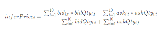
The linear regression slope of the top-10 weighted average price refers to the slope of the linear regression of the top-10 weighted average price with respect to time t.
Net Buy Increase in the Best 10 Bids
The net buy increase in the best 10 bid orders measures the overall increase in bid-side capital within the effective price range, calculated as the total sum of changes in bid prices:
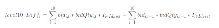
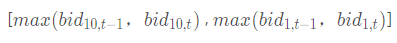
The effective price range refers to the valid price within the following ranges:
2.2 Factor Implementation in DolphinDB
Linear Regression Slope of Top-10 Weighted Average Price
The calculation of the slope of the linear regression of the top-10 weighted average price requires the following four fields, all of which are array vector storing the volumes/prices in one column:
- OfferOrderQty: Volumes of ten lowest sell orders
- BidOrderQty: Volumes of ten highest buy orders
- OfferPrice: Prices of ten lowest sell orders
- BidPrice: Prices of ten highest buy orders
The rowSum built-in aggregate function can be used to calculate
the sum of each row efficiently. The linearTimeTrend function
computes the sliding linear regression slope with respect to time t, returning
both the intercept and slope of the regression.
price.ffill().linearTimeTrend(lag1-1).at(1).nullFill(0).mavg(lag2,
                        1).nullFill(0)
calculates the slope of the linear regression of the
top-10 weighted average price.
@state
def level10_InferPriceTrend(bid, ask, bidQty, askQty, lag1=60, lag2=20){
	inferPrice = (rowSum(bid*bidQty)+rowSum(ask*askQty))\(rowSum(bidQty)+rowSum(askQty))
	price = iif(bid[0] <=0 or ask[0]<=0, NULL, inferPrice)
	return price.ffill().linearTimeTrend(lag1-1).at(1).nullFill(0).mavg(lag2, 1).nullFill(0)
}
Net Buy Increase in the Best 10 Bids
The calculation of the net buy increase in the best 10 bid orders requires two array vector fields:
- BidOrderQty – Volumes of ten highest buy orders
- BidPrice – Prices of ten highest buy orders
The rowAlign function aligns the current and previous best 10
prices. The rowAt and nullFill functions are
then used to align the corresponding order quantities and prices. Finally, the
total change is calculated.
@state
def level10_Diff(price, qty, buy, lag=20){
        prevPrice = price.prev()
        left, right = rowAlign(price, prevPrice, how=iif(buy, "bid", "ask"))
        qtyDiff = (qty.rowAt(left).nullFill(0) - qty.prev().rowAt(right).nullFill(0))
        amtDiff = rowSum(nullFill(price.rowAt(left), prevPrice.rowAt(right)) * qtyDiff)
        return msum(amtDiff, lag, 1).nullFill(0)
}
2.3 Factor Implementation in Python
Linear Regression Slope of Top-10 Weighted Average Price
def level10_InferPriceTrend(df, lag1=60, lag2=20):
    '''
    Linear Regression Slope of Top-10 Weighted Average Price
    :param df:
    :param lag1:
    :param lag2:
    :return:
    '''
    temp = df[["SecurityID","DateTime"]]
    temp["amount"] = 0.
    temp["qty"] = 0.
    for i in range(10):
        temp[f"bidAmt{i+1}"] = df[f"BidPrice{i+1}"].fillna(0.) * df[f"BidOrderQty{i+1}"].fillna(0.)
        temp[f"askAmt{i+1}"] = df[f"OfferPrice{i+1}"].fillna(0.) * df[f"OfferOrderQty{i+1}"].fillna(0.)
        temp["amount"] += temp[f"bidAmt{i+1}"] + temp[f"askAmt{i+1}"]
        temp["qty"] += df[f"BidOrderQty{i+1}"].fillna(0.) + df[f"OfferOrderQty{i+1}"].fillna(0.)
    temp["inferprice"] = temp["amount"] / temp["qty"]
    temp.loc[(temp.bidAmt1 <= 0) | (temp.askAmt1 <= 0), "inferprice"] = np.nan
    temp["inferprice"] = temp["inferprice"].fillna(method='ffill').fillna(0.)
    def f(x):
        n = len(x)
        x = np.array(x)
        y = np.array([i for i in range(1, n+1)])
        return (n*sum(x*y) - sum(x)*sum(y)) / (n*sum(y*y) - sum(y)*sum(y))
    temp["inferprice"] = temp.groupby("SecurityID")["inferprice"].apply(lambda x: x.rolling(lag1 - 1, 1).apply(f))
    temp["inferprice"] = temp["inferprice"].fillna(0)
    temp["inferprice"] = temp.groupby("SecurityID")["inferprice"].apply(lambda x: x.rolling(lag2, 1).mean())
    return temp[["SecurityID","DateTime", "inferprice"]].fillna(0)
Net Buy Increase in the Best 10 Bids
def level10_Diff(df, lag=20):
    '''
    Net Buy Increase in the Best 10 Bids
    :param df:
    :param lag:
    :return:
    '''
    temp = df[["SecurityID","DateTime"]]
    for i in range(10):
        temp[f"bid{i+1}"] = df[f"BidPrice{i+1}"].fillna(0)
        temp[f"bidAmt{i+1}"] = df[f"BidOrderQty{i+1}"].fillna(0) * df[f"BidPrice{i+1}"].fillna(0)
        temp[f"prevbid{i+1}"] = temp[f"bid{i+1}"].shift(1).fillna(0)
        temp[f"prevbidAmt{i+1}"] = temp[f"bidAmt{i+1}"].shift(1).fillna(0)
    temp["bidMin"] = temp[[f"bid{i+1}" for i in range(10)]].min(axis=1)
    temp["bidMax"] = temp[[f"bid{i+1}" for i in range(10)]].max(axis=1)
    temp["prevbidMin"] = temp[[f"prevbid{i+1}" for i in range(10)]].min(axis=1)
    temp["prevbidMax"] = temp[[f"prevbid{i+1}" for i in range(10)]].max(axis=1)
    temp["pmin"] = temp[["bidMin", "prevbidMin"]].max(axis=1)
    temp["pmax"] = temp[["bidMax", "prevbidMax"]].max(axis=1)
    temp["amtDiff"] = 0.0
    for i in range(10):
        temp["amtDiff"] += temp[f"bidAmt{i+1}"]*((temp[f"bid{i+1}"] >= temp["pmin"])&(temp[f"bid{i+1}"] <= temp["pmax"])).astype(int) - \
                        temp[f"prevbidAmt{i+1}"]*((temp[f"prevbid{i+1}"] >= temp["pmin"])&(temp[f"prevbid{i+1}"] <= temp["pmax"])).astype(int)
    temp["amtDiff"] = temp.groupby("SecurityID")["amtDiff"].apply(lambda x: x.rolling(lag, 1).sum())
    return temp[["SecurityID","DateTime", "amtDiff"]].fillna(0)
3. Calculation Results
3.1 Calculation Performance
The daily volume of Level-2 market snapshot data exceeds 10 GB, making the calculation performance of high-frequency factors based on this data a key concern for practitioners. This section compares the calculation performance of the two high-frequency factors from two perspectives: We adjusted the level of parallelism by varying the number of CPU cores used and measured the time taken to compute the factors under different storage formats. The test data consists of 26,632 securities with a total of 31 million rowsfor one trading day. All tests were conducted after clearing the operating system cache. The test results are summarized in the following tables:
| Storage Format\Factor | Linear Regression Slope of the Top-10 Weighted Average Price(s) | Net Buy Increase in the Best 10 Bids(s) |
|---|---|---|
| DolphinDB | 2.4 | 2.3 |
| Python+pickle | 254.3(104.8×) | 105.9(45.4×) |
| Python+parquet | 309.4(127.5×) | 147.9(63.4×) |
| Python+feather | 291.1(120.0×) | 130.6(56.0×) |
| Python+Hdf5 | 281.4(116.0×) | 132.0(56.6×) |
| Python+Npz | 346.7(142.9×) | 175.2(75.1×) |
| Storage Format\Factor | Linear Regression Slope of the Top-10 Weighted Average Price(s) | Net Buy Increase in the Best 10 Bids(s) |
|---|---|---|
| DolphinDB | 4.5 | 4.4 |
| Python+pickle | 489.3(102.8×) | 231.6(60.0×) |
| Python+parquet | 638.7(143.0×) | 296.3(67.9×) |
| Python+feather | 594.2(133.1×) | 261.9(60.0×) |
| Python+Hdf5 | 563.4(126.2×) | 294.6(67.5×) |
| Python+Npz | 648.7(145.3×) | 334.3(76.6×) |
| Storage Format\Factor | Linear Regression Slope of the Top-10 Weighted Average Price(s) | Net Buy Increase in the Best 10 Bids(s) |
|---|---|---|
| DolphinDB | 6.5 | 6.8 |
| Python+pickle | 1014.9(155.6×) | 363.9(53.6×) |
| Python+parquet | 1134.9(174.0×) | 560.9(82.6×) |
| Python+feather | 1040.6(159.6×) | 479.7(70.7×) |
| Python+Hdf5 | 1021.2(156.6×) | 437.4(64.4×) |
| Python+Npz | 1260.3(193.2×) | 638.8(94.1×) |
| Storage Format\Factor | Linear Regression Slope of the Top-10 Weighted Average Price(s) | Net Buy Increase in the Best 10 Bids(s) |
|---|---|---|
| DolphinDB | 21.8 | 22.0 |
| Python+pickle | 3638.2(166.5×) | 1461.8(66.3×) |
| Python+parquet | 4450.4(203.7×) | 1759.3(79.8×) |
| Python+feather | 3994.0(182.8×) | 1773.7(80.5×) |
| Python+Hdf5 | 3996.9(182.9×) | 1774.5(80.5×) |
| Python+Npz | 5031.4(230.3×) | 2437.3(110.6×) |
These tables present the performance improvement of factor calculations with different numbers of CPU cores. DolphinDB's integrated factor calculations achieve up to 200× performance improvement for the linear regression slope of the top-10 weighted average price compared to Python-based calculations using various file storage formats, with an average improvement of approximately 100×. The performance advantages of DolphinDB's integrated calculations can be attributed to the following factors:
- DolphinDB’s proprietary data storage system provides significantly higher data retrieval efficiency compared to Python reading general file formats.
- DolphinDB’s built-in functions, such as
rowSumandlinearTimeTrend, eliminate the need for complexforloop-based calculations, significantly reducing computational time.
Although file formats such as Pickle and Parquet can be optimized through technical methods (e.g., redundant storage), it often results in higher hardware resource costs and increased data management complexity. In contrast, DolphinDB's proprietary storage system is more efficient, user-friendly, and simpler to manage. DolphinDB’s integrated factor calculation framework demonstrates significantly faster processing speed—from data loading to factor calculation—compared to Python + file storage solutions. There are several key insights from the performance comparison:
- Implementation: DolphinDB’s SQL-based calculation framework simplifies factor calculation and parallel execution.
- Parallelism: DolphinDB automatically utilizes available CPU resources, whereas Python scripts require explicit parallel scheduling, which offers more flexibility but demands additional coding effort.
- Speed: DolphinDB’s integrated calculation is 50 to 200× faster than Python + file storage solutions.
3.2 Accuracy Comparison
While DolphinDB's integrated factor calculation is significantly faster than Python + file storage, we must also consider the accuracy of the results. To verify consistency, the calculation results from both solutions were respectively imported into Pandas DataFrames for comparison. The code comparing the results of the DolphinDB solution and the Python+Pickle solution is shown below, which makes it easy to see that the results of both solutions are exactly the same:
from pandas.testing import assert_frame_equal
df_ddb = df_dolphindb.sort_values(by=["SecurityID","DateTime","amtDiff"]).reset_index(drop=True)
df_py = res_combined.sort_values(by=["SecurityID","DateTime","amtDiff"]).reset_index(drop=True)
df_ddb = df_ddb.round(4)
df_py = df_py.round(4)
assert_frame_equal(df_ddb, df_py, check_exact=False, rtol=1, atol=1e-06)
print(assert_frame_equal)
"""
The assert_frame_equal function does not produce any output when the results match.
If the results do not match, it returns an error message.
"""
4. FAQ
How to Reproduce the Code in This Article?
Follow the steps below to set up and run the project:
Step 1: DolphinDB Deployment
First, download and deploy a standalone DolphinDB server. This step can be performed on both Linux and Windows systems. For detailed guidance, refer to the following link:
Standalone Deployment and Upgrade
Step 2: DolphinDB Client Installation
Install and launch the DolphinDB GUI or VS Code(with DolphinDB extension installed). After connecting to the server, you can execute the DolphinDB scripts. For detailed guidance, refer to the following links:
Step 3: Upload and Extract Code Package
Upload the file Python_plus_file_VS_dolphindb_on_factor_calc.zip to the server. Use the following commands to move and extract the file on a Linux system:
cd /home/ddb/workfile/demo/
unzip python_plus_file_VS_dolphindb_on_factor_calc.zip -d ./ /home/ddb/workfile/demo/. Modify the path based on your actual
environment.Step 4: Execute DolphinDB and Python Scripts
- Execute
00_dolphindb_script/00_genSimulatedData.dosto generate simulated data. - Execute
00_dolphindb_script/01_saveAsCsv.dosto save the simulated data as CSV files. - Execute
00_dolphindb_script/02_level10Diff.dosto compute the linear regression slope of the top-10 weighted average price in DolphinDB. - Execute
00_dolphindb_script/03_level10InferPriceTrend.dosto compute the net buy increase in the best 10 bid orders in DolphinDB. - Execute
00_python_script/save_given_format_file/04_save_pickle.pyto save CSV files as Pickle files. - Execute
00_python_script/calc_factor/05_level10Diff_pickle.pyto compute the linear regression slope of the top-10 weighted average price in Python. - Execute
00_python_script/calc_factor/06_level10InferPriceTrend_pickle.pyto calculate the net buy increase in the best 10 bid orders in Python.
The example above uses the Pickle files. To test other file formats, run the corresponding file-saving scripts first, followed by the factor calculation scripts.
5. Conclusion
The comparative results in this article demonstrate that, under the condition of using the same number of CPU cores: DolphinDB's integrated factor calculation achieves performance that is approximately 50 to 200 times faster than Python factor calculation solutions using various file storage formats, with identical calculation results.
Data Management & Reading Efficiency
- DolphinDB is a distributed system specifically designed for large-scale data analysis and processing. It employs an efficient columnar storage format to optimize I/O operations. Therefore, DolphinDB exhibits significantly higher performance in reading and writing large datasets compared to the Python Pandas library, which may encounter performance bottlenecks when handling extremely large datasets.
- DolphinDB’s memory management is highly efficient, capable of handling datasets larger than the available memory. This ensures stable and high performance when processing large datasets. In contrast, Python-based processing may require more memory management and optimization work when handling large datasets.
- As a high-performance database, DolphinDB integrates a rich set of API, supports complete version compatibility, and provides robust access control. Using general file storage formats, on the other hand, may face challenges in cross-platform usage, version compatibility, and access control. DolphinDB offers significant advantages in operational efficiency and ease of management over file-based storage solutions.
Factor Implementation
- DolphinDB’s in-memory SQL-based computation framework simplifies factor calculation and parallel execution.
- DolphinDB's built-in functions, like
rowSumandlinearTimeTrend, are optimized for vectorization, significantly improving factor calculation performance by eliminating complex loop-based operations.. The overall code size can be reduced by more than 50%.
Parallelism Management
- DolphinDB can automatically use the available CPU resources, enabling seamless parallel execution. Python scripts, on the other hand, require explicit coding to manage parallel execution, which offers more flexibility but requires additional implementation effort.
In summary, DolphinDB's integrated calculation framework makes it the ideal choice for high-frequency factor calculation in financial applications.