Factor Calculation Solutions Compared: Python + HDF5 vs. DolphinDB
In quantitative trading, calculating high-frequency factors based on L1/L2 market quotes and high-frequency trading data is a common requirement for research and investment strategies. However, the exponential growth in historical L1/L2 market data volumes presents significant challenges for traditional relational databases such as MS SQL Server and MySQL. Even with sharding strategies, these databases often struggle to meet the performance demands of efficient data querying and analysis. As a result, many practitioners have turned to distributed file systems, using HDF5 for data storage and Python for quantitative financial computations.
While HDF5 effectively handles large-scale high-frequency datasets, it introduces several challenges, including complex permission management, difficulties in joining isparate datasets, inefficiencies in data retrieval and querying, and issues related to data redundancy. Additionally, using Python for data processing incurs substantial time overhead due to data transfer bottlenecks.
DolphinDB, an advanced analytical platform powered by a distributed time-series database, has emerged as a preferred solution for many brokerages and private equity firms. This article aims to provide a comparative analysis of the Python + HDF5 factor calculation approach against DolphinDB's integrated factor calculation solution.
1. Testing Environment and Data
1.1 Testing Environment
This test compares factor calculation implementations based on Python + HDF5 and DolphinDB.
- Python + HDF5 Solution: Uses libraries such as Numpy, Pandas, dolphindb, and Joblib.
- DolphinDB Integrated Solution: Uses DolphinDB server as the computational platform, with a single-node deployment for this test.
The hardware and software environment details required for the test are as follows:
Hardware Environment
| Hardware | Configuration |
|---|---|
| CPU | Intel(R) Xeon(R) Silver 4210R CPU @ 2.40GHz |
| Memory | 512 GB |
| Disk | SSD 500 GB |
Software Environment
| Software | Version |
|---|---|
| Operating System | CentOS Linux release 7.9.2009 (Core) |
| DolphinDB | V2.00.8.7 |
| Python | V3.6.8 |
| Numpy | V1.19.3 |
| Pandas | V1.1.5 |
1.2 Test Data
The test dataset consists of snapshot data for three trading days between January 2, 2020, and January 6, 2020. The data covers approximately 1,992 stocks, with an average daily data volume of about 7.6 million records and a total data volume of approximately 22 million records. The original data is stored in DolphinDB, and HDF5 format data files can be exported from DolphinDB for use in the Python + HDF5 solution.
The snapshot table in DolphinDB contains 55 fields, with some key fields displayed as follows:
| Field Name | Data Type |
|---|---|
| TradeDate | DATE |
| OrigTime | TIMESTAMP |
| dbtime | TIMESTAMP |
| SecurityID | SYMBOL |
| OfferPX1 | INT |
| BidPX1 | DOUBLE |
| OfferSize1 | DOUBLE |
| BidSize1 | INT |
| …… | …… |
An exmaple of the snapshot data is as follows:
	TradeDate	OrigTime	SendTime	Recvtime	dbtime	ChannelNo	SecurityID	SecurityIDSource	MDStreamID	OfferPX1	BidPX1	OfferSize1	BidSize1	OfferPX2	BidPX2	OfferSize2	BidSize2	OfferPX3	BidPX3	OfferSize3	BidSize3	OfferPX4	BidPX4	OfferSize4	BidSize4	OfferPX5	BidPX5	OfferSize5	BidSize5	OfferPX6	BidPX6	OfferSize6	BidSize6	OfferPX7	BidPX7	OfferSize7	BidSize7	OfferPX8	BidPX8	OfferSize8	BidSize8	OfferPX9	BidPX9	OfferSize9	BidSize9	OfferPX10	BidPX10	OfferSize10	BidSize10	NUMORDERS_B1	NOORDERS_B1	ORDERQTY_B1	NUMORDERS_S1	NOORDERS_S1	ORDERQTY_S1
0	2020.01.02	2020.01.02 09:00:09.000	2020.01.02 09:00:09.264	2020.01.02 09:00:09.901	202.01.02 09:00:09.902	1,014	000014	102	010	0	0	0	0	0	0	0	0	0	0	0	0	0	0	0	0	0	0	0	0	0	0	0	0	0	0	0	0	0	0	0	0	0	0	0	0	0	0	0	0	0	0		0	0
1	2020.01.02	2020.01.02 09:01:09.000	2020.01.02 09:01:09.330	2020.01.02 09:01:09.900	2020.01.02 09:01:09.904	1,014	000014	102	010	0	0	0	0	0	0	0	0	0	0	0	0	0	0	0	0	0	0	0	0	0	0	0	0	0	0	0	0	0	0	0	0	0	0	0	0	0	0	0	0	0	0		0	0
2	2020.01.02	2020.01.02 09:02:09.000	2020.01.02 09:02:09.324	2020.01.02 09:02:10.131	2020.01.02 09:02:10.139	1,014	000014	102	010	0	0	0	0	0	0	0	0	0	0	0	0	0	0	0	0	0	0	0	0	0	0	0	0	0	0	0	0	0	0	0	0	0	0	0	0	0	0	0	0	0	0		0	0
3	2020.01.02	2020.01.02 09:03:09.000	2020.01.02 09:03:09.223	2020.01.02 09:03:10.183	2020.01.02 09:03:10.251	1,014	000014	102	010	0	0	0	0	0	0	0	0	0	0	0	0	0	0	0	0	0	0	0	0	0	0	0	0	0	0	0	0	0	0	0	0	0	0	0	0	0	0	0	0	0	0		0	0
4	2020.01.02	2020.01.02 09:04:09.000	2020.01.02 09:04:09.227	2020.01.02 09:04:10.188	2020.01.02 09:04:10.215	1,014	000014	102	010	0	0	0	0	0	0	0	0	0	0	0	0	0	0	0	0	0	0	0	0	0	0	0	0	0	0	0	0	0	0	0	0	0	0	0	0	0	0	0	0	0	0		0	0
5	2020.01.02	2020.01.02 09:05:09.000	2020.01.02 09:05:09.223	2020.01.02 09:05:09.930	2020.01.02 09:05:09.936	1,014	000014	102	010	0	0	0	0	0	0	0	0	0	0	0	0	0	0	0	0	0	0	0	0	0	0	0	0	0	0	0	0	0	0	0	0	0	0	0	0	0	0	0	0	0	0		0	0
6	2020.01.02	2020.01.02 09:06:09.000	2020.01.02 09:06:09.218	2020.01.02 09:06:10.040	2020.01.02 09:06:10.044	1,014	000014	102	010	0	0	0	0	0	0	0	0	0	0	0	0	0	0	0	0	0	0	0	0	0	0	0	0	0	0	0	0	0	0	0	0	0	0	0	0	0	0	0	0	0	0		0	0
7	2020.01.02	2020.01.02 09:07:09.000	2020.01.02 09:07:09.224	2020.01.02 09:07:09.922	2020.01.02 09:07:09.925	1,014	000014	102	010	0	0	0	0	0	0	0	0	0	0	0	0	0	0	0	0	0	0	0	0	0	0	0	0	0	0	0	0	0	0	0	0	0	0	0	0	0	0	0	0	0	0		0	0
8	2020.01.02	2020.01.02 09:08:09.000	2020.01.02 09:08:09.220	2020.01.02 09:08:10.137	2020.01.02 09:08:10.154	1,014	000014	102	010	0	0	0	0	0	0	0	0	0	0	0	0	0	0	0	0	0	0	0	0	0	0	0	0	0	0	0	0	0	0	0	0	0	0	0	0	0	0	0	0	0	0		0	0
9	2020.01.02	2020.01.02 09:09:09.000	2020.01.02 09:09:09.215	2020.01.02 09:09:10.175	2020.01.02 09:09:10.198	1,014	000014	102	010	0	0	0	0	0	0	0	0	0	0	0	0	0	0	0	0	0	0	0	0	0	0	0	0	0	0	0	0	0	0	0	0	0	0	0	0	0	0	0	0	0	0		0	0
2. Factor Code Implementation
This section compares the implementation of two high-frequency factors—Flow Factor and mathWghtSkew Factor—in DolphinDB and Python.
2.1 High-Frequency Factors
Flow Factor
The Flow Factor relies on historical data and requires four fields: buy_vol,
sell_vol, askPrice1, and bidPrice1. It uses functions such as
mavg and iif to calculate the flow of
buyer funds.

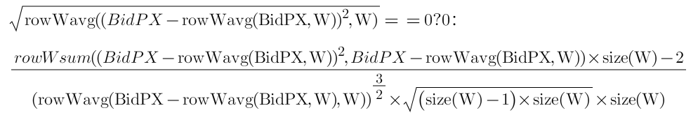
mathWghtSkew Factor
This factor processes multi-level quote data (e.g., BidPX1, BidPX2, ..., BidPX10) and calculates the weighted skewness of the quotes.
2.2 Factor Implementation in DolphinDB
DolphinDB provides optimized functions for time-series calculations, such as
mavg (moving average) and rowWavg
(row-weighted average). These functions simplify the development of
high-frequency factors and deliver excellent computational performance.
Flow Factor Implementation Code:
def flow(buy_vol, sell_vol, askPrice1, bidPrice1){
	buy_vol_ma = round(mavg(buy_vol, 60), 5)
	sell_vol_ma = round(mavg(sell_vol, 60), 5)
	buy_prop = iif(abs(buy_vol_ma+sell_vol_ma) < 0, 0.5 , buy_vol_ma/ (buy_vol_ma+sell_vol_ma))
	spd_tmp = askPrice1 - bidPrice1
	spd = iif(spd_tmp  < 0, 0, spd_tmp)
	spd_ma = round(mavg(spd, 60), 5)
	return iif(spd_ma == 0, 0, buy_prop / spd_ma)
}
mathWghtSkew Factor Implementation Code:
def mathWghtCovar(x, y, w){
	v = (x - rowWavg(x, w)) * (y - rowWavg(y, w))
	return rowWavg(v, w)
}
def mathWghtSkew(x, w){
	x_var = mathWghtCovar(x, x, w)
	x_std = sqrt(x_var)
	x_1 = x - rowWavg(x, w)
	x_2 = x_1*x_1
	len = size(w)
	adj = sqrt((len - 1) * len) \ (len - 2)
	skew = rowWsum(x_2, x_1) \ (x_var * x_std) * adj \ len
	return iif(x_std==0, 0, skew)
}
2.3 Factor Implementation in Python
In Python, the implementation relies on libraries such as NumPy and Pandas.
Flow Factor Implementation Code:
def flow(df):
    buy_vol_ma = np.round(df['BidSize1'].rolling(60).mean(), decimals=5)
    sell_vol_ma = np.round((df['OfferSize1']).rolling(60).mean(), decimals=5)
    buy_prop = np.where(abs(buy_vol_ma + sell_vol_ma) < 0, 0.5, buy_vol_ma / (buy_vol_ma + sell_vol_ma))
    spd = df['OfferPX1'].values - df['BidPX1'].values
    spd = np.where(spd < 0, 0, spd)
    spd = pd.DataFrame(spd)
    spd_ma = np.round((spd).rolling(60).mean(), decimals=5)
    return np.where(spd_ma == 0, 0, pd.DataFrame(buy_prop) / spd_ma)
mathWghtSkew Factor Implementation Code:
def rowWavg(x, w):
    rows = x.shape[0]
    res = [[0]*rows]
    for row in range(rows):
        res[0][row] = np.average(x[row], weights=w)
    res = np.array(res)
    return res
def rowWsum(x, y):
    rows = x.shape[0]
    res = [[0]*rows]
    for row in range(rows):
        res[0][row] = np.dot(x[row],y[row])
    res = np.array(res)
    return res
def mathWghtCovar(x, y, w):
    v = (x - rowWavg(x, w).T)*(y - rowWavg(y, w).T)
    return rowWavg(v, w)
def mathWghtSkew(x, w):
    x_var = mathWghtCovar(x, x, w)
    x_std = np.sqrt(x_var)
    x_1 = x - rowWavg(x, w).T
    x_2 = x_1*x_1
    len = np.size(w)
    adj = np.sqrt((len - 1) * len) / (len - 2)
    skew = rowWsum(x_2, x_1) / (x_var*x_std)*adj / len
    return np.where(x_std == 0, 0, skew)
2.4 Summary
From the perspective of code implementation, there is little difference in
difficulty between developing these factors in DolphinDB and Python. The
implementation is straightforward in DolphinDB with its built-in functions. The
sliding window calculations in Python are performed using combinations of
functions like rolling and mean. In DolphinDB,
similar calculations can be achieved using the moving function
combined with functions like mean or avg.
However, such combinations may lack incremental optimization due to the lack of
specific business context. To enhance performance, DolphinDB provides
specialized moving window functions (e.g., mavg), which can be
optimized for specific computational needs. These optimized functions can
improve performance by up to 100 times compared to generic combinations.
3. Factor Calculation Performance
This chapter further demonstrates how to invoke calculations of these factors and implement parallel calculations in DolphinDB and Python.
3.1 Factor Calculation in DolphinDB
Factor Calculation
In DolphinDB, the Flow Factor requires moving window calculations, while the
mathWghtSkew Factor involves multi-column calculations within the same row.
These calculations are performed independently for each stock. DolphinDB
simplifies such operations with the context by clause, which
allows batch processing of time-series data for multiple stocks. By using
context by on the stock SecurityID,
DolphinDB's SQL engine can directly perform batch moving window calculations for
multiple stocks. The calculation code is as follows:
m = 2020.01.02:2020.01.06
w = 10 9 8 7 6 5 4 3 2 1
res = select dbtime, SecurityID,flow(BidSize1,OfferSize1, OfferPX1, BidPX1) as Flow_val,mathWghtSkew(matrix(BidPX1,BidPX2,BidPX3,BidPX4,BidPX5,BidPX6,BidPX7,BidPX8,BidPX9,BidPX10),w) as Skew_val  from loadTable("dfs://LEVEL2_SZ","Snap") where TradeDate between  m context by SecurityID
Parallel Execution
DolphinDB's computational framework breaks down computation jobs into smaller tasks for parallel execution. Therefore, when executing the above SQL, DolphinDB automatically identifies the data partitions and performs multi-threaded parallel calculations based on the configured parameter workerNum. This parameter can be modified in the DolphinDB configuration file. Users can control the CPU resource utilization and parallelism during factor calculations. The parallelism of the current task in DolphinDB can be viewed through the web interface.
3.2 Factor Calculation in Python
HDF5 Data File Reading
Unlike DolphinDB's in-database calculations, Python requires reading snapshot
data from HDF5 files before performing computations. Two common methods for
reading HDF5 files in Python are pandas.HDFStore() and
pandas.read_hdf(). While read_hdf()
supports reading specific columns, the performance difference between reading
partial and full columns is minimal. Additionally, HDF5 files saved using
pandas.to_hdf() consume about 30% more storage space than
those saved using pandas.HDFStore(). Due to the larger storage
space, reading the same HDF5 data using pandas.read_hdf() takes
longer than using pandas.HDFStore(). Therefore, this test uses
pandas.HDFStore() for storing and reading HDF5 file data.
The HDF5 files in this test are stored in the most generic way, without
redundancy removal or other storage optimizations, as such optimizations
increase data usage and management complexity, especially in massive data
scenarios.
Saving and Reading HDF5 Files
# Save HDF5 file
def saveByHDFStore(path,df):
    store = pd.HDFStore(path)
    store["Table"] = df
    store.close()

# Read a single HDF5 file
def loadData(path):
    store = pd.HDFStore(path, mode='r')
    data = store["Table"]
    store.close()
    return data
Factor Calculation
For each stock, daily data is read in a loop, concatenated into a DataFrame, and factor calculations are performed.
def ParallelBySymbol(SecurityIDs,dirPath):
    for SecurityID in SecurityIDs:
        sec_data_list=[]
        for date in os.listdir(dirPath):
            filepath = os.path.join(dirPath,str(date),"data_"+str(date) + "_" + str(SecurityID) + ".h5")
            sec_data_list.append(loadData(filepath))
        df=pd.concat(sec_data_list)
        # Calculate Flow Factor
        df_flow_res = flow(df)
        # Calculate mathWghtSkew
        w = np.array([10, 9, 8, 7, 6, 5, 4, 3, 2, 1])
        pxs = np.array(df[["BidPX1","BidPX2","BidPX3","BidPX4","BidPX5","BidPX6","BidPX7","BidPX8","BidPX9","BidPX10"]])
        np.seterr(divide='ignore', invalid='ignore')
        df_skew_res = mathWghtSkew(pxs,w)
Parallel Scheduling
We use Python's Joblib library to implement multi-process
parallel scheduling. The stocks to be calculated are read from files and split
into multiple groups based on the parallelism level.
# Stock HDF5 file directory
pathDir = "/data/stockdata"
# Parallelism level
n = 1
# SecurityIDs is the list of all stocks to be calculated
SecurityIDs_splits = np.array_split(SecurityIDs, n)
Parallel(n_jobs=n)(delayed(ParallelBySymbol)(SecurityIDs, pathDir) for SecurityIDs in SecurityIDs_splits)
3.3 Validation of Calculation Results
We stored the factor calculation results from both Python + HDF5 and DolphinDB in DolphinDB's distributed tables. A full data comparison was performed using the following code to validate consistency between calculation results.
resTb = select * from loadTable("dfs://tempResultDB", "result_cyc_test")
resTb2 = select * from loadTable("dfs://tempResultDB", "result_cyc_test2")
resTb.eq(resTb2).matrix().rowAnd().not().at()
An output of int[0] indicates that the contents of the two
tables are identical.
3.4 Performance Comparison
The performance of Python + HDF5 and DolphinDB is compared under different parallelism levels using a dataset of 1,992 stocks over 3 days (22 million records). The time consumption (in seconds) is measured for different numbers of CPU cores. All tests are performed after flushing the operating system cache.
| CPU Cores | Python + HDF5 | DolphinDB | (Python + HDF5) / DolphinDB |
|---|---|---|---|
| 1 | 2000 | 21.0 | 95 |
| 2 | 993 | 11.5 | 86 |
| 4 | 540 | 6.8 | 79 |
| 8 | 255 | 5.8 | 44 |
| 16 | 133 | 4.9 | 27 |
| 24 | 114 | 4.3 | 26 |
| 40 | 106 | 4.2 | 25 |
From the results, we observe that DolphinDB's in-database calculations can reach nearly 100 times faster than Python + HDF5 calculations under single-core conditions. As the number of CPU cores increases, the performance ratio stabilizes at around 1:25.
DolphinDB's proprietary storage system is significantly more efficient than Python's generic HDF5 file reading. While HDF5 files can be optimized for storage performance, this comes with additional hardware resource costs and increased data management complexity. In contrast, DolphinDB's storage system is designed for high efficiency, ease of use, and seamless integration with its analytical capabilities.
From the perspective of code implementation and optimizaiton, DolphinDB provides
optimized moving window functions which deliver superior performance for moving
calculations compared to Python's standard rolling()
operations. Additionally, DolphinDB's in-database SQL-based calculations
simplify factor implementation and enable seamless parallel execution. While
DolphinDB automatically utilizes available CPU resources, Python requires
explicit parallel scheduling code, which provides finer control over concurrency
but also increases implementation complexity.
4. Conclusion
This article compares the performance, development efficiency, and data management capabilities of DolphinDB and the Python + HDF5 solution for high-frequency factor calculations. The comparison results in this article demonstrate that, under the condition of using the same number of CPU cores:
Performance
DolphinDB's in-database calculations are approximately 25 times faster than the Python + HDF5 factor calculation solution, while producing identical results to the Python approach.
Development Efficiency
Both solutions offer similar ease of factor implementation, though DolphinDB benefits from built-in optimized functions that reduce the need for custom parallelization.
Data Management & Reading Efficiency
HDF5 files operate in a single-threaded manner for reading and writing, making parallel data operations difficult. Data retrieval efficiency in HDF5 depends heavily on the file’s internal organizational structure (groups and datasets). Optimizing read/write performance often requires custom storage design, sometimes involving redundant data storage to meet different access needs. As data volumes grow to the terabyte level, HDF5 data management complexity increases significantly, leading to substantial time and storage costs in practical use.
In contrast, DolphinDB simplifies data storage, querying, and management through its efficient storage engines and partitioning mechanisms. Users can easily manage and utilize data at the petabyte scale and beyond, similar to operating a conventional database.