DolphinDB Application in Deep Learning: Real-Time Stock Volatility Prediction
Deep learning, a branch of machine learning, employs multi-layer neural networks to automatically extract features from data and excels particularly in handling complex data such as images, text, and time-series data. In finance, deep learning is well-suited to modeling nonlinear relationships and high-dimensional datasets, offering strong capabilities in market prediction and pattern recognition. Consider algorithmic trading: it has progressed through four major generations, with the current AI-driven phase distinguished by the use of advanced deep learning models to generate signals and guide trade execution.
Although deep learning demonstrates tremendous potential in quantitative finance, several practical challenges remain:
- Storage and computation of large-scale features (factors)
- Real-time streaming computation of factors
- Engineering integration of factor data with deep learning models
As a high-performance time-series database integrating distributed computing, storage, and real-time stream processing, DolphinDB is highly suitable for factor storing, computing, modeling, backtesting, and live trading. It effectively addresses the first two challenges by supporting large-scale factor computation, storage, and real-time updates. Meanwhile, to solve the third challenge, DolphinDB provides tools such as the AI DataLoader and Libtorch plugin, enabling seamless integration with deep learning frameworks like PyTorch and TensorFlow. These tools combine DolphinDB's data processing power with deep learning capabilities for efficient model inference and analysis.
This document uses real-time stock volatility prediction as a case study to demonstrate DolphinDB’s capabilities across the deep learning workflow—including high-frequency factor storage and computation, model training using AI DataLoader in Python, and real-time prediction via the Libtorch plugin in DolphinDB. The focus is on illustrating the operational process rather than optimizing predictive accuracy; the model and results are for demonstration purposes only.
Complete code and partial sample data are provided to help readers follow the tutorial. Refer to the appendix for the development environment used. While GPU versions of DolphinDB and the Libtorch plugin are used here, the same code can also run on CPU versions.
1. Overview
Using AI algorithmic trading as an example, it mainly consists of two phases: algorithm research and live trading. Each phase has different priorities in terms of technology stack selection. This chapter first examines the strengths and limitations of common existing solutions, followed by an introduction to a streamlined, one-stop solution based on DolphinDB.
1.1 Existing Solutions
In the research phase, typical technology stack includes NAS files + HDFS clusters + Python. Python offers a rich ecosystem for data science and machine learning, but its global interpreter lock (GIL) limits parallel computation. While frameworks such as Ray can provide distributed computing support, they introduce additional system complexity and maintenance overhead. Frequent access to high-frequency data is also common in research. Though NAS and HDFS are designed for large-scale storage, they often fall short in scalability, performance, and availability as data volumes and computational demands grow. Moreover, this setup usually requires substantial secondary development and ongoing maintenance.
In live trading, stream calculation of real-time factors poses further challenges in balancing performance and efficiency. Python supports full computation but lacks efficient incremental processing, making it unsuitable for low-latency applications. To meet production performance needs, many institutions re-implement research code in C++, resulting in duplicated development efforts and increased maintenance. Additionally, considerable effort is required to ensure the results of the two codebases are fully consistent.
1.2 DolphinDB Solution
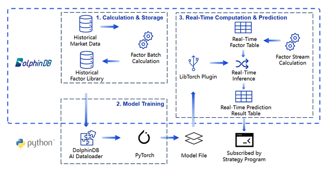
To address these challenges, DolphinDB offers a unified solution. Historical market data is stored in DolphinDB’s distributed database, supporting high-speed, large-scale factor computation. In the Python environment, the AI DataLoader enables seamless loading of factor data from DolphinDB into tensors compatible with frameworks like PyTorch, facilitating model training. After training, models can be used for inference directly within DolphinDB via the Libtorch plugin. Together with DolphinDB’s high-performance stream tables and real-time computing engines, this setup enables fast processing of live data, generation of real-time factor tables, and prediction outputs. Ultimately, the real-time prediction result table can be subscribed to by strategy programs such as those written in Python for subsequent signal processing and other operations, completing the full algorithm execution pipeline. The specific process is shown in the diagram below:
2. Factor Calculation and Storage
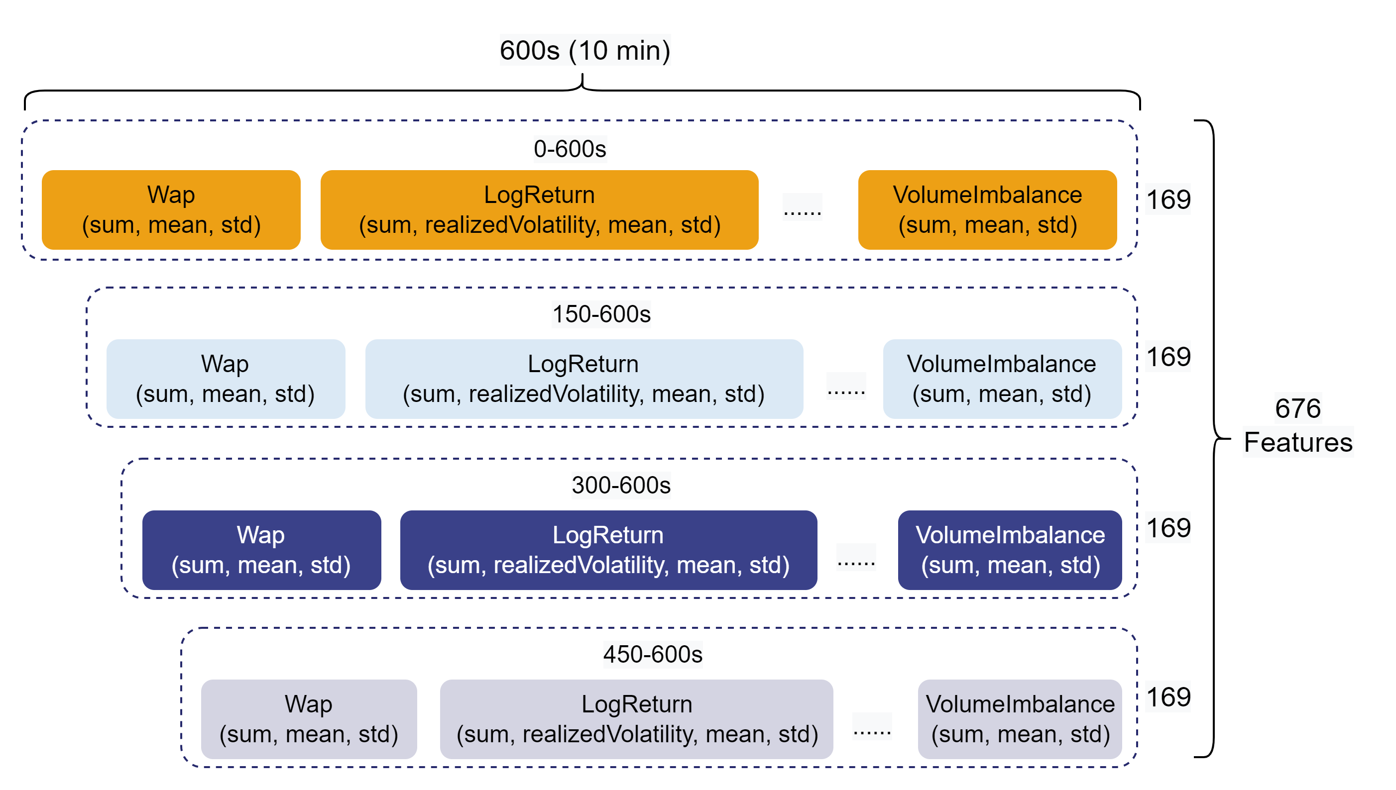
This chapter is based on the tutorial Feature Engineering for Stock Volatility Prediction, using Level-2 snapshot data of stocks (sampled every 3 seconds) to construct multi-frequency features in DolphinDB. Through metaprogramming, 676 derived feature columns are generated with minimal code, and the results are stored in a DolphinDB database for later use in model training.
The structure of the snapshot data is as follows:
| Field | Description | Field | Description | Field | Description |
|---|---|---|---|---|---|
| SecurityID | Stock code | LowPx | Lowest price | BidPrice[10] | Top 10 bid prices |
| DateTime | Timestamp | LastPx | Latest price | BidOrderQty[10] | Top 10 bid volumes |
| PreClosePx | Previous close | TotalVolumeTrade | Cumulative volume | OfferPrice[10] | Top 10 ask prices |
| OpenPx | Opening price | TotalValueTrade | Cumulative turnover | OfferOrderQty[10] | Top 10 ask volumes |
| HighPx | Highest price | InstrumentStatus | Trading status | … | … |
The dataset contains Level-2 snapshots of all stocks on a specific exchange throughout 2021, totaling approximately 1.7 billion records, pre-imported into DolphinDB. To support hands-on practice, one month of snapshot data for a single stock is provided in the appendix, along with scripts for database/table creation and data import. Note that full-year data is used for model training, while only a subset is included in the appendix due to size limitations.
2.1 Factor Calculation
Feature engineering is a key component of quantitative research. As the scale of quantitative strategies and AI models expands, developers must manage increasingly large volumes of factor data. In this example, primary and secondary indicators are derived from the best 10 bid/ask prices and volumes in the Level-2 data. These indicators are then aggregated over 10-minute intervals, with four overlapping segments for each interval: 0–600s, 150–600s, 300–600s, and 450–600s, producing 676-dimensional feature vectors.
All 676 factors are generated dynamically via metaprogramming, with fewer than 70 lines of code. Compared to running parallelized Pandas processes in Python, DolphinDB’s distributed computing delivers up to 30x better performance. Partial sample code is as follows:
// Define aggregation function
defg featureEngineering(DateTime, BidPrice, BidOrderQty, OfferPrice, OfferOrderQty, aggMetaCode){
	wap = (BidPrice * OfferOrderQty + BidOrderQty * OfferPrice) \ (BidOrderQty + OfferOrderQty)
	wapBalance = abs(wap[0] - wap[1])
	priceSpread = (OfferPrice[0] - BidPrice[0]) \ ((OfferPrice[0] + BidPrice[0]) \ 2)
	BidSpread = BidPrice[0] - BidPrice[1]
	OfferSpread = OfferPrice[0] - OfferPrice[1]
	totalVolume = OfferOrderQty.rowSum() + BidOrderQty.rowSum()
	volumeImbalance = abs(OfferOrderQty.rowSum() - BidOrderQty.rowSum())
	logReturnWap = logReturn(wap)
	logReturnOffer = logReturn(OfferPrice)
	logReturnBid = logReturn(BidPrice)
	subTable = table(DateTime as `DateTime, BidPrice, BidOrderQty, OfferPrice, OfferOrderQty, wap, wapBalance, priceSpread, BidSpread, OfferSpread, totalVolume, volumeImbalance, logReturnWap, logReturnOffer, logReturnBid)
	colNum = 0..9$STRING
	colName = `DateTime <- (`BidPrice + colNum) <- (`BidOrderQty + colNum) <- (`OfferPrice + colNum) <- (`OfferOrderQty + colNum) <- (`Wap + colNum) <- `WapBalance`PriceSpread`BidSpread`OfferSpread`TotalVolume`VolumeImbalance <- (`logReturn + colNum) <- (`logReturnOffer + colNum) <- (`logReturnBid + colNum)
	subTable.rename!(colName)
	subTable['BarDateTime'] = bar(subTable['DateTime'], 10m)
	result = sql(select = aggMetaCode, from = subTable).eval().matrix()
	result150 = sql(select = aggMetaCode, from = subTable, where = <time(DateTime) >= (time(BarDateTime) + 150*1000) >).eval().matrix()
	result300 = sql(select = aggMetaCode, from = subTable, where = <time(DateTime) >= (time(BarDateTime) + 300*1000) >).eval().matrix()
	result450 = sql(select = aggMetaCode, from = subTable, where = <time(DateTime) >= (time(BarDateTime) + 450*1000) >).eval().matrix()
	return concatMatrix([result, result150, result300, result450])
}

// Generate and query with metaprogramming
whereConditions = [<date(DateTime) between 2021.01.04 : 2021.12.31>, <SecurityID in stockList>, <(time(DateTime) between 09:30:00.000 : 11:29:59.999) or (time(DateTime) between 13:00:00.000 : 14:56:59.999)>]
result = sql(select = sqlColAlias(<featureEngineering(DateTime, matrix(BidPrice), matrix(BidOrderQty), matrix(OfferPrice), matrix(OfferOrderQty), aggMetaCode)>, metaCodeColName <- (metaCodeColName+"_150") <- (metaCodeColName+"_300") <- (metaCodeColName+"_450")), from = snapshot, where = whereConditions, groupBy = [<SecurityID>, <bar(DateTime, 10m) as DateTime>]).eval()
2.2 Factor Storage
Efficient factor storage is essential for scalable quantitative research. DolphinDB supports two storage formats: wide-format tables and narrow-format tables. Compared to wide format, narrow format offers better performance for adding, updating, and deleting individual factors. For storing 10-minute frequency features, extensive testing (see the Optimal Storage for Trading Factors Calculated at Mid to High Frequencies tutorial) supports the following configuration as a best practice:
- Partitioning scheme: COMPO-partitioned by month and factor name
- Storage engine: TSDB
- Sort columns: SecurityID + DateTime
create database "dfs://tenMinutesFactorDB"
partitioned by VALUE(2021.01M..2021.12M), VALUE(`f1`f2)
engine = 'TSDB'

create table "dfs://tenMinutesFactorDB"."tenMinutesFactorTB"(
	SecurityID SYMBOL,
	DateTime TIMESTAMP[comment="time column", compress="delta"],
	FactorNames SYMBOL,
	FactorValues DOUBLE
)
partitioned by DateTime, FactorNames,
sortColumns=[`SecurityID, `DateTime],
keepDuplicates=ALL,
sortKeyMappingFunction=[hashBucket{, 500}]
3. Model Building and Training
This chapter uses Python to load feature data from the DolphinDB database via the AI
DataLoader and invokes the PyTorch framework to train a deep learning model to
predict 10-minute future volatility. In financial markets, volatility is commonly
used to measure the degree of change in stock prices over time. Therefore, the
variable LogReturn0_realizedVolatility is selected as the target
value for model prediction. In the following sections, we include only the key code
snippets relevant to the integration between DolphinDB and the model training
pipeline.
3.1 Loading Training Data with AI Dataloader
The AI DataLoader (DDBDataLoader) is used to load training data from DolphinDB and convert it into tensor formats compatible with deep learning frameworks like PyTorch. With AI DataLoader, users can avoid manually implementing a custom Dataset class. Instead, data can be efficiently loaded using SQL queries executed directly on the DolphinDB server. AI DataLoader optimizes performance by splitting SQL queries into smaller subqueries, minimizing memory usage on the client side and improving control over data loading.
Installation
First, install the DolphinDB Python API and its deep learning toolkit
DDBDataLoader.
pip install dolphindb
pip install dolphindb-tools
Data Preprocessing and Splitting
The following Python code connects to the DolphinDB server and preprocesses the data:
# Data preprocessing and splitting into training and testing sets
conn = ddb.session("192.168.100.201", 8848, "admin", "123456")
conn.run("""startDay = 2021.01.01
            endDay = 2021.12.31
            splitDay = (startDay..endDay)[((endDay-startDay)*0.8).floor()]
            Data = select FactorValues from loadTable("dfs://tenMinutesFactorDB", "tenMinutesFactorTB") where date(DateTime) >= objByName('startDay') and date(DateTime) <= objByName('endDay') and SecurityID=`600030 pivot by DateTime, SecurityID, FactorNames
            Data = Data[each(isValid, Data.values()).rowAnd()]
            """)
The code above connects to the DolphinDB database for data preprocessing.
Through the conn.run interface, the script is sent to the
DolphinDB server for execution. In this example, factor data from 2021.01.01 to
2021.12.31 is used, and the dataset is split into training and test sets at an
8:2 ratio based on date. The pivot by statement converts the
narrow-format factors into a wide format for easier tensor conversion.
Additionally, rows with missing values in factor columns are removed. Optional
preprocessing steps, such as normalization or standardization, can also be
applied here if required.
Initializing AI DataLoader
Next, two DDBDataloader objects are instantiated, one for
loading training data and the other for testing. The only difference between
them is the sql parameter, which specifies different time ranges.
# Dataloader parameters
targetColumns = ["LogReturn0_realizedVolatility"]
excludedColumns = ["SecurityID", "DateTime", "LogReturn0_realizedVolatility"]
batchSize = 256
windowSize = [120, 1]
windowStride=[1, 1]
offset = 120
trainSql = """select * from objByName('Data') where date(DateTime) >= objByName('startDay') and date(DateTime) <= objByName('splitDay')"""
testSql = """select * from objByName('Data') where date(DateTime) > objByName('splitDay') and date(DateTime) <= objByName('endDay')"""

# Instantiate DDBDataloader
trainLoader = DDBDataLoader(ddbSession=conn, sql=trainSql, targetCol=targetColumns, excludeCol=excludedColumns, batchSize=batchSize, device=device, windowSize=windowSize, windowStride=windowStride, offset=offset)
testLoader = DDBDataLoader(ddbSession=conn, sql=testSql, targetCol=targetColumns, excludeCol=excludedColumns, batchSize=batchSize, device=device, windowSize=windowSize, windowStride=windowStride, offset=offset)
print("Using DDBDataLoader, data is ready")- ddbSession: Session connection used to obtain data, including contextual information required for training.
- sql: Metacode of SQL statements to extract data for training. The DDBDataLoader object splits the query into multiple subqueries based on database partitions. Internally, threads in DDBDataLoader convert and stitch the split data into the format required by PyTorch training, which is then placed into a prefetch queue.
- targetCol: Target column (i.e., the target variable for model prediction), which is set to LogReturn0_realizedVolatility.
- excludeCol: Columns to be excluded by x in the iteration. Here, SecurityID, DateTime, and LogReturn0_realizedVolatility are excluded to ensure they are not used as input features.
- batchSize: Number of messages in each batch of data, which is 256.
- windowSize: Size of the sliding window. It is set to [120, 1], meaning each input sample consists of 120 time points of factor sequence data, and the target corresponds to 1 time point.
- windowStride: Step of the sliding window. It is set to [1, 1], meaning the window moves forward by 1 time point each time.
- offset: Offset between the input and target data. It is set to 120, indicating that the target is the value 120 time points after the input.
- device: Whether to load data to GPU or CPU.
With these settings, AI DataLoader efficiently extracts and formats the time-series factor data for model training (e.g., LSTM or other sequence models). Support for sliding windows significantly simplifies feature engineering for temporal prediction tasks.
3.2 Model Building
The objective of this training task is to predict stock volatility, which exhibits strong temporal dependencies. To effectively capture these sequential patterns, an LSTM network is employed.
# Model definition
class LSTMModel(nn.Module):
    def __init__(self, inputSize, units):
        super(LSTMModel, self).__init__()
        self.lstm1 = nn.LSTM(input_size=inputSize, hidden_size=units, batch_first=True, dropout=0.4)
        self.lstm2 = nn.LSTM(input_size=units, hidden_size=128, batch_first=True, dropout=0.3)
        self.lstm3 = nn.LSTM(input_size=128, hidden_size=32, batch_first=True, dropout=0.1)
        self.fc = nn.Linear(32, 1)

    def forward(self, x):
        out, _ = self.lstm1(x)
        out, _ = self.lstm2(out)
        out, _ = self.lstm3(out)
        out = out[:, -1, :]
        out = self.fc(out)
        return out
3.3 Model Training
The training process using AI DataLoader closely resembles that of PyTorch’s native DataLoader. Below is the training loop example:
# Training phase
model.train()
trainLoss = 0.0
trainLen = 0
for inputs, targets in trainLoader:
    inputs = inputs.float().to(device)
    targets = targets.float().to(device)
    optimizer.zero_grad()
    outputs = model(inputs)
    loss = criterion(outputs, targets)
    trainLoss += loss.item()
    loss.backward()
    optimizer.step()
    trainLen += 1
trainLoss /= trainLen
The model iterates over batches fetched from trainLoader,
calculates the loss and updates weights using the optimizer.
After training, the model is saved in TorchScript format so it can be deployed within DolphinDB via the Libtorch plugin:
torchScriptModel = torch.jit.script(model)
torchScriptModel.save("/your_path/LSTMmodel.pt")
3.4 Training Performance
Using 10-minute factor data of one year for a single stock, the LSTM model is trained over 100 epochs, with a total training time of 72 seconds. The test hardware/software is provided in the appendix. Details of the test are as follows:
- Total dataset volume: 5832 rows (one year of 10-minute data).
- Number of features: 676 factors (input dimension: 675, target dimension: 1).
- Data preprocessing:
- Data is filtered by date range (from January 1 to December 31, 2021).
- Data is processed using a sliding window with window size 120, stride 1, and target offset 120.
- Model architecture:
- Three-layer LSTM with hidden units 256, 128, and 32 respectively.
- The output layer is a fully connected layer with output dimension 1.
- Dropout is used to prevent overfitting (LSTM1: 0.4, LSTM2: 0.3, LSTM3: 0.1).
- Loss function:
SmoothL1Loss. - Optimizer: Adam with an initial learning rate of 0.0001.
- Batch size: 256.
- Number of training epochs: 100.
- Device: NVIDIA GPU.
4. Real-Time Computation and Prediction
The previous sections focused on batch processing of historical data. In production, market data arrives in real time as streams. This section demonstrates how to extend earlier feature engineering and modeling scripts for streaming computation and real-time prediction using DolphinDB’s time-series engine and Libtorch plugin.
We simulate real-time input by replaying one day of historical snapshot data at 100x speed from the database. First, a stream table is created to receive replayed data:
name = loadTable("dfs://l2StockSHDB", "snapshot").schema().colDefs.name
type = loadTable("dfs://l2StockSHDB", "snapshot").schema().colDefs.typeString
share(streamTable(100000:0, name, type), `SnapshotStream)
Then, implement the computation logic and subscribe to raw snapshot data. The following example replays one day of snapshot data for a single stock at 100x speed.
testSnapshot = select * from loadTable("dfs://l2StockSHDB", "snapshot") where SecurityID=`600030 and date(DateTime)=mdDate
submitJob("replaySnapshot", "replay 1 day snapshot", replay{testSnapshot, SnapshotStream, `DateTime, `DateTime, 100, false, 1, , true})
4.1 Streaming Real-Time Factor Computation
One way DolphinDB achieves unified batch-stream processing is by applying functions or expressions to calculating high-frequency financial factors using different computation engines for historical or streaming data. In this example, we reuse all factor functions defined in Section 2.1. In batch processing, the factor functions were passed into the SQL engine to compute historical data. In stream processing, we pass them into the streaming engine to process real-time data.
// Create real-time factor table
share(streamTable(100000:0 , `DateTime`SecurityID`ReceiveTime <- metaCodeColName <- (metaCodeColName+"_150") <- (metaCodeColName+"_300") <- (metaCodeColName+"_450") <- `HandleTime,`TIMESTAMP`SYMBOL`NANOTIMESTAMP <- take(`DOUBLE, 676) <- `NANOTIMESTAMP) , `aggrFeatures10min)
go
// Create time-series engine
metrics=sqlColAlias(<featureEngineering(DateTime,
		matrix(BidPrice[0],BidPrice[1],BidPrice[2],BidPrice[3],BidPrice[4],BidPrice[5],BidPrice[6],BidPrice[7],BidPrice[8],BidPrice[9]),
		matrix(BidOrderQty[0],BidOrderQty[1],BidOrderQty[2],BidOrderQty[3],BidOrderQty[4],BidOrderQty[5],BidOrderQty[6],BidOrderQty[7],BidOrderQty[8],BidOrderQty[9]),
		matrix(OfferPrice[0],OfferPrice[1],OfferPrice[2],OfferPrice[3],OfferPrice[4],OfferPrice[5],OfferPrice[6],OfferPrice[7],OfferPrice[8],OfferPrice[9]),
		matrix(OfferOrderQty[0],OfferOrderQty[1],OfferOrderQty[2],OfferOrderQty[3],OfferOrderQty[4],OfferOrderQty[5],OfferOrderQty[6],OfferOrderQty[7],OfferOrderQty[8],OfferOrderQty[9]), aggMetaCode)>, metaCodeColName <- (metaCodeColName+"_150") <- (metaCodeColName+"_300") <- (metaCodeColName+"_450"))

createTimeSeriesEngine(name="aggrFeatures10min", windowSize=600000, step=600000, metrics=[<now(true) as ReceiveTime>, metrics, <getHandleTime() as HandleTime>], useSystemTime=false ,dummyTable=SnapshotStream, outputTable=aggrFeatures10min, timeColumn=`DateTime, useWindowStartTime=true, keyColumn=`SecurityID)
// Subscribe to raw market data and write to the aggregation engine in real time
subscribeTable(tableName="SnapshotStream", actionName="aggrFeatures10min", offset=-1, handler=getStreamEngine("aggrFeatures10min"), msgAsTable=true, batchSize=2000, throttle=0.01, hash=0, reconnect=true)
The above script creates a time-series engine for streaming factor computation and subscribes to the SnapshotStream table to write data into the engine in real time. The engine aggregates incoming snapshot data, caches necessary historical data, and continuously writes computed factors to the aggrFeatures10min stream table.
4.2 Real-Time Model Inference Using Libtorch Plugin
DolphinDB provides the Libtorch plugin, which allows directly loading and using TorchScript models within the DolphinDB environment. We subscribe to the output table of the time-series engine created in the previous section, process real-time and historical features into the model’s input format (tensor), and perform inference.
First, install and load the Libtorch plugin. The CPU version plugin is called "Libtorch", while the GPU version is "GpuLibtorch" (Note that these two plugins cannot be loaded simultaneously). In this example, the DolphinDB server uses the GPU version (Shark), so the GpuLibtorch plugin is selected.
installPlugin("GpuLibtorch")
loadPlugin("GpuLibtorch")
Next, load the trained model and use setDevice to move the model
to the GPU:
// Load model
modelPath = "/home/lnfu/ytxie/LSTMmodel.pt"
model = Libtorch::load(modelPath)
Libtorch::setDevice(model, "CUDA")
After successfully loading the model trained in Python, subscribe to the
aggrFeatures10min stream table for real-time model inference. Each time new data
arrives in the aggrFeatures10min, the predictRV function is
triggered, and the result is written into the result10min stream table.
// Create real-time prediction result table
share(streamTable(100000:0 , `Predicted`SecurityID`DateTime`ReceiveTime`HandleTime`PredictedTime, `FLOAT`SYMBOL`TIMESTAMP`NANOTIMESTAMP`NANOTIMESTAMP`NANOTIMESTAMP), `result10min)
go
// Define real-time handler: data preprocessing and model inference
def predictRV(model, window, msg){
	tmp = select * from msg
	tmp.dropColumns!(`ReceiveTime`HandleTime)
	tmp.reorderColumns!(objByName(`historyData).columnNames())
	predictedtSet = []
	for(row in tmp){
		objByName(`historyData).tableInsert(row)
		data = tail(objByName(`historyData), window)
		data.dropColumns!(`SecurityID`DateTime`LogReturn0_realizedVolatility)
		data = data[each(isValid, data.values()).rowAnd()]
		input = tensor([matrix(data)$FLOAT])
		predict = Libtorch::predict(model, input)
		predictedtSet.append!(predict[0][0])
	}
	ret = select predictedtSet as predicted, SecurityID, DateTime, ReceiveTime, HandleTime, now(true) as PredictedTime from msg
	objByName("result10min").append!(ret)
}
// Load the past 20 days of 10-minute factors to prepare historical data for the sliding window
data = select FactorValues from loadTable("dfs://tenMinutesFactorDB", "tenMinutesFactorTB") where date(DateTime) between (mdDate-20):(mdDate-1) and SecurityID=`600030 pivot by DateTime, SecurityID, FactorNames
data = data[each(isValid, data.values()).rowAnd()]
share(data, `historyData)
// Window size: use 120 time points to predict the next one
window = 120
// Warm up the model to reduce initial latency
warmupData = tail(objByName(`historyData), window)
warmupData.dropColumns!(`SecurityID`DateTime`LogReturn0_realizedVolatility)
input = tensor([matrix(warmupData)$FLOAT])
out = Libtorch::predict(model, input)
// Subscribe to real-time factor table
subscribeTable(tableName="aggrFeatures10min", actionName="predictRV", offset=-1, handler=predictRV{model, window}, msgAsTable=true, batchSize=100, throttle=0.001, hash=1, reconnect=true)
We retrieve the past 20 days of 10-minute factors from the database to prepare
model input data. Since the model uses 120 time points of 676-dimensional
features as one sample, this historical data is needed during real-time
prediction. In the predictRV function, we concatenate current
and historical data and use tail to take the last 120
records.
Note: The 676 feature dimensions must be in the same order as during
Python training. We use the reorderColumns! function to ensure
the correct order from the engine output.
Before real-time prediction, the model is called once for warm-up.
This step is optional but helps improve real-time inference performance.
Due to CUDA initialization, GPU warm-up, and model loading, the first inference
can incur higher latency. Skipping this warm-up may result in significant delay
when predictRV is triggered for the first time.
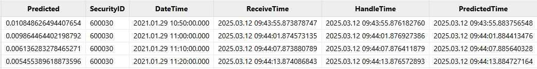
An example of the result is shown in the following figure:
4.3 Real-time Prediction Subscription via Python API
In Python, real-time prediction results can be subscribed using the
subscribe method provided by DolphinDB Python API.
# Subscribe to real-time result stream table
import dolphindb as ddb

s = ddb.session(keepAliveTime=60)
s.connect("192.168.100.201", 8848, "admin", "123456")
s.enableStreaming()

def handler(lst):
    print(lst)

s.subscribe(host="192.168.100.201", port=8848, handler=handler, tableName="result10min", actionName="result10min", offset=-1, resub=True, msgAsTable=True, batchSize=100, throttle=0.001)
The output result upon successful subscription is as follows:

4.4 Real-Time Prediction Performance
The real-time prediction time cost mainly consists of real-time factor computation and model inference. In this example, we use timestamps at each stage to measure the time taken. The factor computation time is obtained by subtracting ReceiveTime from HandleTime. The model inference time is computed as the difference between PredictedTime and HandleTime.
We tested the real-time prediction latency for a single stock using an LSTM model, with one day’s original snapshot data replayed at 100x speed. The total latency per inference is approximately 9.8 milliseconds.
| Average Latency (ms) | 95th Percentile Latency (ms) | Min Latency (ms) | Max Latency (ms) |
|---|---|---|---|
| Factor Computation | 2 | 2 | 2 |
| Model Inference | 7.5 | 8.7 | 7 |
| Total Latency | 9.8 | 10.7 | 9 |
Script for performance statistics:
stat = select (HandleTime-ReceiveTime)/1000/1000 as factorDelay, (PredictedTime-HandleTime)/1000/1000  as predictDelay, (PredictedTime-ReceiveTime)/1000/1000  as totalDelay  from result10min
select avg(factorDelay), percentile(factorDelay, 95), min(factorDelay), max(factorDelay), avg(predictDelay), percentile(predictDelay, 95), min(predictDelay), max(predictDelay), avg(totalDelay), percentile(totalDelay, 95), min(totalDelay), max(totalDelay)  from stat
5. Conclusion
This tutorial presents a complete real-time deep learning solution for stock volatility prediction using DolphinDB. By leveraging its powerful distributed computing, time-series processing, and plugin extensibility, DolphinDB supports low-latency end-to-end AI workflows. Users can adapt and expand the solution to fit their specific business requirements in production environments.
Appendix
Development Environment:
- CPU: AMD EPYC 7513 32-Core Processor @ 2.60GHz
- Logical CPUs: 128
- GPU: NVIDIA A800 80GB PCIe
- Disk: 1 × NVMe
- CUDA Version: 12.4
- Operating System: 64-bit CentOS Linux 7 (Core)
- DolphinDB Version: 3.00.2.3 (2024.11.04), LINUX_ABI x86_64, Shark edition
- DolphinDB Python API Version: 3.0.2.3
- Python Version: 3.12.9
Scripts:
- Database and Table Creation & Data Import: snapshotDB.dos
- Feature Factor Calculation and Storage: FeatureEngineering.dos
- Model Training: LSTMmodel.py
- Real-time Inference: StreamComputing.dos
Data:
- Level-2 Snapshot Data: Snapshot.csv