Best Practices for High-Frequency Backtesting of Market-Making Strategies in Cryptocurrency

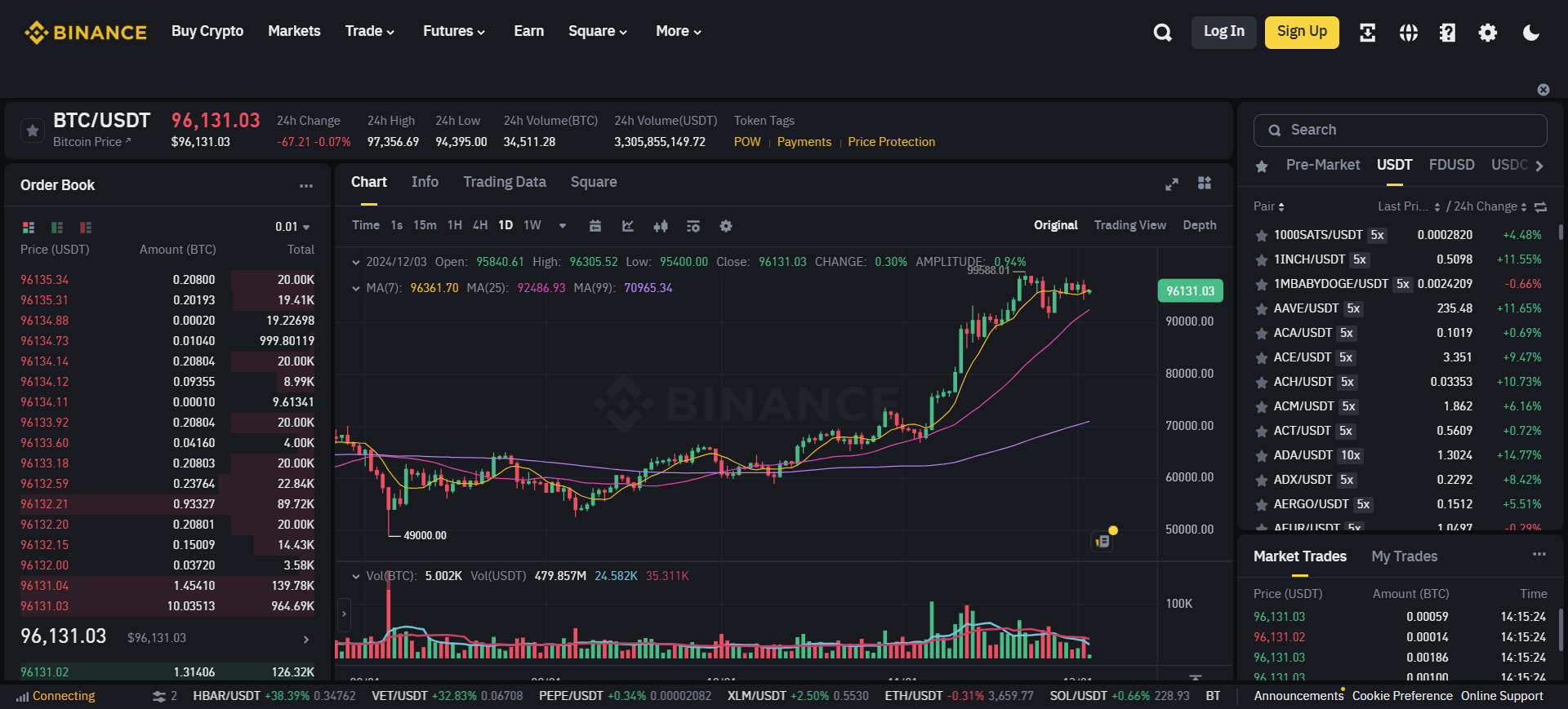
BTC/USDT is a trading pair that represents the price relationship between Bitcoin (BTC) and Tether (USDT), which is commonly regarded as a benchmark for Bitcoin’s price. For example, as shown in the figure below (captured from Binance in December 2024), the BTC/USDT price is 96,191.03, meaning it costs 96,191.03 USDT to purchase 1 BTC.

A perpetual contract is a type of financial derivative based on digital assets, allowing traders to take leveraged long or short positions without holding the underlying asset. Perpetual contracts differ from traditional futures contracts with key features:

• No expiration: Unlike traditional futures commodities, perpetual contracts have no delivery date, allowing traders to hold positions indefinitely.
• Funding rate mechanism: Designed to align contract prices with spot prices, adjusting incentives between longs and shorts. If the funding rate is positive (longs pay shorts), this means the perpetual contract price is higher than the spot price, and long traders need to pay a fee to short traders, and vice versa. Position holders pay or receive the funding rate every 8 hours.
• High leverage: Exchanges offer leverage ranging from 1x to up to 125x.

Market makers provide liquidity by quoting both buy and sell prices, profiting from the bid-ask spread. This tutorial implements the Avellaneda-Stoikov (AS) market-making model for BTC/USDT perpetual contracts.

Cryptocurrency backtesting evaluates a trading strategy performance using historical market data. By simulating trading activity, key metrics such as return, maximum drawdown, and win rate can be calculated to estimate live trading potential. Given the 24/7 nature and high volatility of the cryptocurrency market, particular attention should be paid during backtesting to data quality, trading frequency, fees, slippage, and appropriate risk control measures to handle extreme market conditions and more accurately assess the strategy performance.

DolphinDB provides a simulated matching engine and backtest engine that allow custom strategies to be tested on historical data to evaluate their performance and robustness.

• Simulated matching engine: uses market data and user orders as input, applies matching rules, and outputs execution results to the order detail table. Orders that are not filled immediately are retained for matching with future market data or user cancellation.
• Backtest engine: executes the strategy and risk control management based on historical market data to evaluate strategy performance on historical data, including order generation, matching, capital management, and performance metrics such as return and trade details.

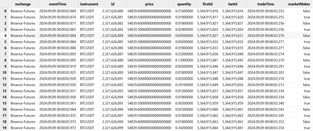
The data structure for USDT-margined aggregated trade data is as follows:

colNames = ["eventTime", "code", "id", "price", "quantity", "firstId", "lastId", 
            "tradeTime", "marketMaker", "currentTime"]
colTypes = [TIMESTAMP, SYMBOL, LONG, DOUBLE, DOUBLE, LONG, LONG,
            TIMESTAMP, BOOL, TIMESTAMP]
trade = table(1:0, colNames, colTypes)

Sample data is as shown below:

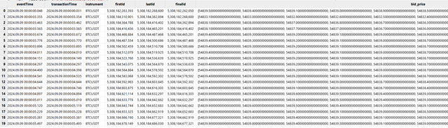
The data structure for the 500-level order book data of USDT-margined contracts is as follows:

colNames = ["eventTime", "transactionTime", "code", "lastUpdateId", "bidPrice", 
              "bidQty", "askPrice", "askQty", "currentTime"]
colTypes = [TIMESTAMP, TIMESTAMP, SYMBOL, LONG, DOUBLE[], 
              DOUBLE[], DOUBLE[], DOUBLE[], TIMESTAMP]
orderbook = table(10000000:0, colNames, colTypes)

Sample data is as shown below:

In addition to market data, funding rates should be considered when trading perpetual contracts as these rates impact a strategy’s capital cost and profitability. DolphinDB’s httpClient plugin supports retrieving real-time or historical funding rate data. The implementation is as follows:

def getBinanceFundingRate(param){
    baseUrl = 'https://fapi.binance.com/fapi/v1/fundingRate'
    config = dict(STRING, ANY)
    //Set to your proxy address
    config[`proxy] = "http://localhost:8899/" 
    response = httpClient::httpGet(baseUrl,param,10000,,config)
    result = fromStdJson(response.text)
    colNames = `symbol`fundingTime`fundingRate`markPrice
    colTypes = [SYMBOL,TIMESTAMP,DECIMAL128(8),DECIMAL128(8)]
    fundingRate = table(1:0, colNames, colTypes)
    for(r in result){//r = result[0]
        r = select string(symbol), timestamp(long(fundingTime)), 
                  decimal128(fundingRate,8), decimal128(markPrice,8) 
            from r.transpose()
        fundingRate.tableInsert(r)
    }
    return fundingRate
}
// params
startDate = 2024.09.09
param = dict(STRING, ANY)
param["symbol"] = 'BTCUSDT'
param["startTime"] = long(timestamp(startDate))
param["endTime"] = long(timestamp(startDate+1)) // Get one-day data
param["limit"] = 1000
fundingRate = select symbol, 
                  fundingTime as settlementTime, 
                  decimal128(fundingRate,8) as lastFundingRate 
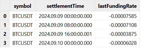
              from getBinanceFundingRate(param)

The data structure is as follows:

colNames = ["symbol", "settlementTime", "lastFundingRate"]
colTypes = [SYMBOL, TIMESTAMP, DECIMAL128(8)]
fundingRate = table(100:0, colNames, colTypes)

Sample data is as shown below:

Before initiating a cryptocurrency backtest, ensure that your DolphinDB version is 3.00.2 or above.

// Prepare Plugins
installPlugin("MatchingEngineSimulator")
installPlugin("Backtest")
try{loadPlugin("Backtest")}catch(ex){print(ex)}
try{loadPlugin("MatchingEngineSimulator")}catch(ex){print(ex)}

Raw market data needs to be cleaned and transformed before it can be used for backtesting. Preprocessing includes but is not limited to removing erroneous data, filling missing values, and aligning data frequency to ensure data quality and consistency. The backtest engine requires snapshot market data schema as follows:

colName = ["symbol", "symbolSource", "timestamp", "tradingDay", "lastPrice", 
          "upLimitPrice", "downLimitPrice", "totalBidQty", "totalOfferQty",
          "bidPrice", "bidQty", "offerPrice", "offerQty", 
          "highPrice", "lowPrice", "signal", "prevClosePrice",
          "settlementPrice", "prevSettlementPrice", "contractType"]
colType =  ["STRING", "STRING", "TIMESTAMP", "DATE", "DECIMAL128(8)", 
          "DECIMAL128(8)", "DECIMAL128(8)", "DECIMAL128(8)", "DECIMAL128(8)",
          "DECIMAL128(8)[]", "DECIMAL128(8)[]", "DECIMAL128(8)[]","DECIMAL128(8)[]",
          "DECIMAL128(8)", "DECIMAL128(8)", "DOUBLE[]", "DECIMAL128(8)",
          "DECIMAL128(8)", "DECIMAL128(8)", "INT"]
messageTable = table(10000000:0, colName, colType)

Since the aggregated trade and order book data obtained from Binance differ from this required format, transformation is necessary. DolphinDB’s built-in wj function can be used to join the aggregated trade data with the order book data, forming the structure required by the backtest engine. Missing fields are filled as appropriate.

def createSnapshotMartketData(orderbook, trade){
        // window join
        messageTable = wj(
              orderbook, trade, 0:0, 
              <[last(price) as lastPrice, 
                sum(bidQty) as totalBidQty, 
                sum(OfferQty) as totalOfferQty, 
                max(price) as highPrice, 
                min(price) as lowPrice]>, 
              `transactionTime, 
              `tradeTime)
        // fill the missing columns
        signal = take(array(DOUBLE[], 0).append!(0), count(messageTable))
        messageTable = select 
                          instrument as symbol, 
                          exchange as symbolSource, 
                          transactionTime as timestamp, 
                          date(transactionTime) as tradingDay, 
                          lastPrice, 
                          decimal128(0, 8) as upLimitPrice, 
                          decimal128(0, 8) as downLimitPrice, 
                          totalBidQty, totalOfferQty, 
                          bid_price as bidPrice, 
                          bid_qty as bidQty, 
                          ask_price as offerPrice, 
                          ask_qty as offerQty, 
                          highPrice, lowPrice, signal, 
                          decimal128(0, 8) as prevClosePrice, 
                          decimal128(0, 8) as settlementPrice, 
                          decimal128(0, 8) as prevSettlementPrice, 
                          2 as contractType 
                    from messageTable
        update messageTable set lastPrice = ffill(lastPrice)
        update messageTable set lastPrice = bfill(lastPrice)
        update messageTable set totalBidQty = nullFill(totalBidQty, 0), 
                                totalOfferQty = nullFill(totalBidQty, 0)
        return messageTable
}
messageTable = createSnapshotMartketData(orderbook, trade)

Configuring the backtest engine includes setting the time range, trading costs, and other parameters. These configurations define the basic conditions for backtesting and how trades are executed. Note:

• dataType is set to 1 with input snapshot data.
• The initial capital cash is defined as a dictionary, with the futures account assumed to hold 1,000,000.
• The funding rate table obtained earlier is input at this step into the backtest engine.

startDate = 2024.09.09
endDate = 2024.09.10
// account
cash = dict(STRING,DOUBLE)
cash["spot"] = 1000000.0
cash["futures"] = 1000000.0
cash["option"] = 1000000.0
// Backtest Engine Configs
userConfig = dict(STRING,ANY)
userConfig["startDate"] = startDate
userConfig["endDate"] = endDate
userConfig["strategyGroup"] = "cryptocurrency"
userConfig["cash"] = cash
userConfig["msgAsTable"] = false 
userConfig["dataType"] = 1 //snapshot
userConfig["matchingMode"] = 3 
userConfig["fundingRate"] = fundingRate

Basic information about each cryptocurrency contract (such as specifications, trading unit, and tick size) must be defined before the backtest begins. The setup of the contract metadata table contractReference can be referred to in the following example.

// Contract Information
contractReference = dict(STRING, ANY)
contractReference["symbol"] = "BTCUSDT"                      // symbol code: BTCUSDT
contractReference["contractType"] = 2                        // contract type: 2 - Perp
contractReference["optType"] = 1                             // option type(Unrelated): set default value, 1
contractReference["strikePrice"] = decimal128(0., 8)   		 // strike price(Unrelated): set default value default Null
contractReference["contractSize"] = decimal128(1. , 8)		 // contract multiplier
contractReference["marginRatio"] = decimal128(0.0065, 8)	 // margin ratio
contractReference["tradeUnit"] = decimal128(1., 8)			 // contract unit
contractReference["priceUnit"] = decimal128(0.1, 8)			 // order unit: 0.1 USDT
contractReference["priceTick"] = decimal128(0.1, 8)	         // minimum order unit: 0.1 USDT
contractReference["takerRate"] = decimal128(0.0005, 8)	     // taker rate
contractReference["makerRate"] = decimal128(0.0002, 8)		 // maker rate
contractReference["deliveryCommissionMode"] = 1       		 // Delivery Fee: 1 - makerRate (or takerRate) per contract
contractReference["fundingSettlementMode"] = 1        		 // Funding Rate Settlement: 1 - lastFundingRate per contract
contractReference["lastTradeTime"] = userParam["endTime"]    // last trading time
// Convert Dict to Table
contractReference = transpose(contractReference)

After completing data preparation and configuration, the next step is to implement the trading strategy, including defining trading signals, entry and exit rules, and stop-loss/take-profit mechanisms.

The logic of this AS strategy is as follows: each time an order is placed, unfilled orders are canceled first. Then, the AS formula is used to calculate the quote, after which buy and sell orders are submitted. A risk management module is also added to close positions in a timely manner.

We input serveral custome parameters to the onSnapshot function, which correspond to the AS model variables. These values can be computed from historical data or updated in real time during trading.

• sigma: market volatility
• gamma: risk aversion coefficient; the closer to 1, the more risk-averse
• k: market liquidity parameter
• amount: order size
• orderInterval: strategy execution frequency (e.g., 5 minutes in milliseconds)

In this strategy, market volatility (sigma) is calculated from the previous day's data as 1.579. The risk aversion coefficient (gamma) is set to 0.1. The market liquidity parameter (k) is set to 0.1, based on the reference from Avellaneda & Stoikov (2008). Each order places 0.01 units, with a strategy frequency of once every 5 minutes. Users can compute, adjust, or optimize these parameters based on their own use case.

sigma = (select std(abs(deltas(price))) as volatility 
          from trade 
          where date(tradeTime) = startDate - 1 
          group by date(tradeTime)
        )[0]["volatility"]
// Onsnapshot Params
userParam = dict(STRING,ANY)
userParam["sigma"] = sigma									// market volatility
userParam["gamma"] = 0.1									// inventory risk aversion parameter
userParam["k"] = 1.5										// order book liquidity parameter
userParam["amount"] = 0.01									// order amount
userParam["endTime"] = endTime								// closing time
userParam["feeRatio"] = 0.0003								// fee ratio
userParam["istock"] = sym									// symbol
userParam["orderTime"] = timestamp(startDate)				// starting time
userParam["orderInterval"] = 1000							// stratygy frequency, ms
userParam["tradeDate"] = date(startDate)					// date
userParam['lastprice'] = last(messageTable["lastPrice"])	// last price
userParam["maxPos"] = 5										// inventory of upper limit
userParam["InventoryTargetPercent"] = 0.2					// target inventory percent 		
userParam["minSpread"] = 0.01	                            // minimum spread

After implementing the strategy, use Backtest::createBacktestEngine to create the engine. Then input data using Backtest::appendQuotationMsg, followed by a termination signal to mark the end of the backtest.

// 1. Create Backtest Engine
strategyName = "marketMakingStrategy"
try{Backtest::dropBacktestEngine(strategyName)}catch(ex){print ex}
engine = Backtest::createBacktestEngine(
										strategyName, 
										userConfig,
										contractReference,
										initialize{,userParam}, 
										beforeTrading,
										,
										onSnapshot,
										onOrder,
										onTrade,
										,
										finalized
									)
// 2. Start backtesting
timer Backtest::appendQuotationMsg(engine, messageTable)
go
endMsg = select top 1* from messageTable where timestamp = max(timestamp)
update endMsg set symbol = "END"
update endMsg set timestamp = endTime
Backtest::appendQuotationMsg(engine,endMsg)
go

The backtest engine simulates order generation, matching, and execution based on the user-provided strategy, and returns trade results and relevant statistics to help evaluate the strategy’s effectiveness.

// Get Result
tradeDetails = Backtest::getTradeDetails(engine)
returnSummary = Backtest::getReturnSummary(long(engine))
context = Backtest::getContextDict(long(engine))
dailyReport = context["dailyReport"]
// Stop backtest
try{Backtest::dropBacktestEngine(strategyName)}catch(ex){print ex}

• Backtest::getTradeDetails(engine) returns detailed trade records.
• Backtest::getReturnSummary(engine) returns a summary of strategy returns.
• Backtest::getContextDict(long(engine)) returns the content of the context.

As can be seen from dailyReport, 184 BTC were bought and 201 BTC sold, yielding a net loss of $27,082.04 and transaction fees totaling $6,489.60.

This high-frequency backtest processes one day of BTC/USDT contract data with one quote per second. The backtest engine completed in 27 seconds.