Stream Processing of Financial Factors
DolphinDB is a high-performance distributed time-series database that combines fast data access with a vectorized, multi-paradigm programming language and powerful computing engines. It supports both the backtesting and development of financial factors as well as real-time streaming processing.
1. Overview
1.1 Stream Processing Framework
DolphinDB's built-in stream processing framework supports the publishing, subscription, preprocessing, and real-time in-memory computation of streaming data. It enables complex factor calculations using rolling windows, sliding windows, and cumulative windows, offering both efficiency and ease of use.
The figure below shows the architecture of the framework:
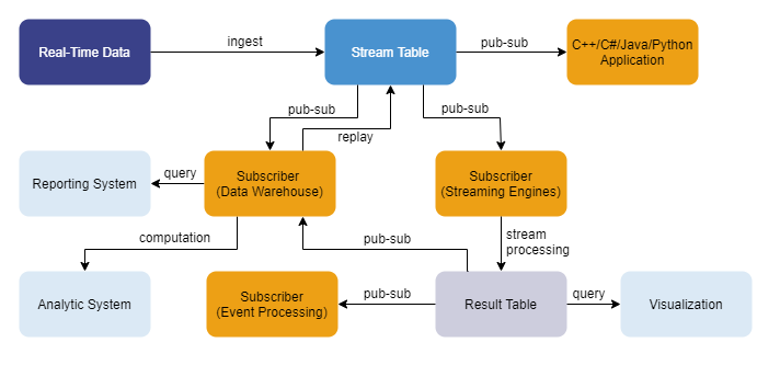
This tutorial focuses on how to use the built-in streaming engines to implement and optimize the computation of factors in quantitative analysis, covering the process of "Stream Table → Subscriber (Streaming Engines) → Result Table."
For details on DolphinDB's built-in streaming engines, see Streaming Engines.
1.2 Data Storage Schemas
The case examples in this tutorial are based on Level 2 market data from a stock exchange. This includes daily OHLC data, tick-by-tick trades, and market snapshots.
Let’s take a look at how DolphinDB stores this data:
(1) Table schema for daily OHLC
| Column Name | Description | Column Name | Description |
|---|---|---|---|
| securityID | Stock Code | lastPx | Closing Price |
| dateTime | Date and Time | volume | Trading Volume |
| preClosePx | Previous Close | amount | Trading Amount |
| openPx | Opening Price | iopv | Net Asset Value |
| highPx | Highest Price | fp_Volume | After-hours Fixed Price Trading Volume |
| lowPx | Lowest Price | fp_Amount | After-hours Fixed Price Trading Amount |
(2) Table schema for tick-by-tick trades
| Column Name | Description | Column Name | Description |
|---|---|---|---|
| securityID | Stock Code | buyNo | Buyer Order Number |
| tradeTime | Date and Time | sellNo | Seller Order Number |
| tradePrice | Transaction Price | tradeBSFlag | Buy/Sell Flag |
| tradeQty | Transaction Volume | tradeIndex | Transaction Sequence Number |
| tradeAmount | Transaction Amount | channelNo | Transaction Channel |
(3) Table schema for Snapshot
DolphinDB provides the array vector structure for storing arrays of varying lengths. Therefore, we have two approaches for storing the top 10 bid/ask prices and their corresponding volumes in market data: either store each price level as separate individual columns, or consolidate them into single array vector columns.


|
Field Name |
Description |
Field Name |
Description |
|---|---|---|---|
|
securityID |
Stock Code |
totalOfferQty |
Total Ask Volume |
|
dateTime |
Date and Time |
weightedAvgBidPx |
Weighted Average Bid Price |
|
preClosePx |
Previous Close Price |
weightedAvgOfferPx |
Weighted Average Ask Price |
|
openPx |
Opening Price |
totalBidNumber |
Total Bid Count |
|
highPx |
Highest Price |
totalOfferNumber |
Total Ask Count |
|
lowPx |
Lowest Price |
bidTradeMaxDuration |
Maximum Wait Time for Bid |
|
lastPx |
Latest Price |
offerTradeMaxDuration |
Maximum Wait Time for Ask |
|
totalVolumeTrade |
Total Trading Volume |
numBidOrders |
Number of Bid Price Levels |
|
totalValueTrade |
Total Trading Amount |
numOfferOrders |
Number of Ask Price Levels |
|
instrumentStatus |
Trading Status |
withdrawBuyNumber |
Number of Buy Withdrawals |
|
bidPrice0 - bidPrice9 (separate columns); bidPrice (array vector) |
Bid Prices (Top 10) |
withdrawBuyAmount |
Volume of Buy Withdrawals |
|
bidOrderQty0 - bidOrderQty9 (separate columns); bidOrderQty (array vector) |
Bid Volumes (Top 10) |
withdrawBuyMoney |
Amount of Buy Withdrawals |
|
bidNumOrders0 - bidNumOrders9 (separate columns); bidNumOrders (array vector) |
Total Bid Orders (Top 10) |
withdrawSellNumber |
Number of Sell Withdrawals |
|
bidOrders0 - bidOrders49 (separate columns); bidOrders (array vector) |
Top 50 Bid Orders |
withdrawSellAmount |
Volume of Sell Withdrawals |
|
offerPrice0 - offerPrice9 (separate columns); offerPrice (array vector) |
Ask Prices (Top 10) |
withdrawSellMoney |
Amount of Sell Withdrawals |
|
offerOrderQty0 - offerOrderQty9 (separate columns); offerOrderQty (array vector) |
Ask Volumes (Top 10) |
etfBuyNumber |
Number of ETF Subscriptions |
|
offerNumOrders0 - offerNumOrders9 (separate columns); offerNumOrders (array vector) |
Total Ask Orders (Top 10) |
etfBuyAmount |
Volume of ETF Subscriptions |
|
offerOrders0 - offerOrders49 (separate columns); offerOrders (array vector) |
Top 50 Ask Orders |
etfBuyMoney |
Amount of ETF Subscriptions |
|
numTrades |
Number of Trades |
etfSellNumber |
Number of ETF Redemptions |
|
iopv |
ETF Net Asset Value |
etfSellAmount |
Volume of ETF Redemptions |
|
totalBidQty |
Total Bid Volume |
etfSellMoney |
Amount of ETF Redemptions |
2. Implementing Daily Frequency Factors
DolphinDB features several built-in streaming engines, including time series, reactive state, and cross-sectional engines. Complex financial factors typically require various computation types—such as cross-sectional analysis, historical state calculation, and time-based window aggregation—which traditionally meant manually connecting multiple streaming engines.
To simplify this process, DolphinDB developed a stream engine parser that automatically analyzes factor expressions and creates optimized engine pipelines, eliminating the need for complex chaining code. For real-time computation of complex daily frequency factors, this stream engine parser offers the most efficient approach.
DolphinDB also provides code implementations of factors from established libraries such as the WorldQuant 101 Alpha Factor Library, encapsulated in the wq101alpha.dos module. These factor implementations work seamlessly in both batch and streaming processing scripts, allowing users to easily implement daily frequency factor streaming calculations via the stream engine parser (through the streamEngineParser function).
In this section, we explore the practical application of automatically constructing engine pipelines through two complex daily frequency factor examples. Then, we explain how the engine parser interprets factor expressions and builds the pipeline, enabling users to apply the parser based on their business needs for enhanced efficiency.
2.1 Examples
We choose two daily frequency factors to demonstrate how they are implemented in real-time in DolphinDB.
2.1.1 Daily Frequency Factor 1
This factor is WorldQuant Alpha#1.
Formulaic expression
(rank(Ts_ArgMax(SignedPower(((returns < 0) ? stddev(returns, 20) : close), 2.), 5)) - 0.5)Code implementation
def wqAlpha1(close){
    ts = mimax(pow(iif(ratios(close) - 1 < 0, mstd(ratios(close) - 1, 20), close), 2.0), 5)
    return rowRank(X=ts, percent=true) - 0.5
}
Stream processing script
// Define input and output schemas
colName = `securityID`dateTime`preClosePx`openPx`highPx`lowPx`lastPx`volume`amount`iopv`fp_Volume`fp_Amount
colType = ["SYMBOL","TIMESTAMP","DOUBLE","DOUBLE","DOUBLE","DOUBLE","DOUBLE","INT","DOUBLE","DOUBLE","INT","DOUBLE"]
inputTable = table(1:0, colName, colType)
resultTable = table(10000:0, ["dateTime", "securityID", "factor"], [TIMESTAMP, SYMBOL, DOUBLE])

// Build engine pipeline using streamEngineParser
try{ dropStreamEngine("alpha1Parser0")} catch(ex){ print(ex) }
try{ dropStreamEngine("alpha1Parser1")} catch(ex){ print(ex) }
metrics = <[securityid, wqAlpha1(preClosePx)]>
streamEngine = streamEngineParser(name="alpha1Parser", metrics=metrics, dummyTable=inputTable, outputTable=resultTable, keyColumn="securityID", timeColumn=`dateTime, triggeringPattern='keyCount', triggeringInterval=3000)

// View created engines
getStreamEngineStat()
/*
ReactiveStreamEngine->
name          user  status lastErrMsg numGroups numRows numMetrics memoryInUsed snapshotDir ...
------------- ----- ------ ---------- --------- ------- ---------- ------------ -----------
alpha1Parser0 admin OK                0         0       2          13392                    ...

CrossSectionalEngine->
name         user  status lastErrMsg numRows numMetrics metrics      triggering...triggering......
------------ ----- ------ ---------- ------- ---------- ------------ --------------- --------------- ---
alpha1Parser1admin OK                0       2          securityid...keyCount     3000         ...
*/
The above script creates an engine pipeline "alpha1Parser." By using the getStreamEngineStat function, we can see that this engine pipeline consists of a reactive state engine "alpha1Parser0" and a cross-sectional engine "alpha1Parser1."
The securityID column is used as grouping key, and dateTime is the time column. The input schema is specified by the in-memory inputTable. The factors to compute are specified in metrics, and the results are stored in the in-memory resultTable. The cross-sectional engine is triggered by “keyCount”, which means a calculation occurs either:
- When the number of keys with the same timestamp reaches 3000 (triggeringInterval)
- When data with a newer timestamp arrives.
Once the engine pipeline is created, insert sample records to view the results:
// Insert data into pipeline
insert into streamEngine values(`000001, 2023.01.01, 30.85, 30.90, 31.65, 30.55, 31.45, 100, 3085, 0, 0, 0)
insert into streamEngine values(`000002, 2023.01.01, 30.86, 30.55, 31.35, 29.85, 30.75, 120, 3703.2, 0, 0, 0)
insert into streamEngine values(`000001, 2023.01.02, 30.80, 30.95, 31.05, 30.05, 30.85, 200, 6160, 0, 0, 0)
insert into streamEngine values(`000002, 2023.01.02, 30.81, 30.99, 31.55, 30.15, 30.65, 180, 5545.8, 0, 0, 0)
insert into streamEngine values(`000001, 2023.01.03, 30.83, 31.00, 31.35, 30.35, 30.55, 230, 7090.9, 0, 0, 0)
insert into streamEngine values(`000002, 2023.01.03, 30.89, 30.85, 31.10, 30.00, 30.45, 250, 7722.5, 0, 0, 0)
insert into streamEngine values(`000001, 2023.01.04, 30.90, 30.86, 31.10, 30.40, 30.75, 300, 9270, 0, 0, 0)
insert into streamEngine values(`000002, 2023.01.04, 30.85, 30.95, 31.65, 30.55, 31.45, 270, 8329.5, 0, 0, 0)
insert into streamEngine values(`000001, 2023.01.05, 30.86, 30.55, 31.35, 29.85, 30.75, 360, 11109.6, 0, 0, 0)
insert into streamEngine values(`000002, 2023.01.05, 30.80, 30.95, 31.05, 30.05, 30.85, 200, 6160, 0, 0, 0)
insert into streamEngine values(`000001, 2023.01.06, 30.81, 30.99, 31.55, 30.15, 30.65, 180, 5545.8, 0, 0, 0)
insert into streamEngine values(`000002, 2023.01.06, 30.83, 31.00, 31.35, 30.35, 30.55, 230, 7090.9, 0, 0, 0)
insert into streamEngine values(`000001, 2023.01.07, 30.89, 30.85, 31.10, 30.00, 30.45, 250, 7722.5, 0, 0, 0)
insert into streamEngine values(`000002, 2023.01.07, 30.90, 30.86, 31.10, 30.40, 30.75, 300, 9270, 0, 0, 0)
insert into streamEngine values(`000001, 2023.01.08, 30.89, 30.85, 31.10, 30.00, 30.45, 250, 7722.5, 0, 0, 0)
insert into streamEngine values(`000002, 2023.01.08, 30.90, 30.86, 31.10, 30.40, 30.75, 300, 9270, 0, 0, 0)

// View results
select factor from resultTable pivot by dateTime, securityID
/*
dateTime                000001 000002
----------------------- ------ ------
2023.01.01T00:00:00.000
2023.01.02T00:00:00.000
2023.01.03T00:00:00.000
2023.01.04T00:00:00.000
2023.01.05T00:00:00.000 0.5    0
2023.01.06T00:00:00.000 0.5    0
2023.01.07T00:00:00.000 0      0.5
*/
2.1.2 Daily Frequency Factor 2
Formulaic expression
(-1 * CORR(RANK(DELTA(LOG(VOLUME),1)),RANK(((CLOSE-OPEN)/OPEN)),6)Code implementation
def gtjaAlpha1(open, close, vol){
	delta = deltas(log(vol))
    return -1 * (mcorr(rowRank(delta, percent=true), rowRank((close - open) \ open, percent=true), 6))
}
Stream processing script
// Define input and output schemas
colName = `securityID`dateTime`preClosePx`openPx`highPx`lowPx`lastPx`volume`amount`iopv`fp_Volume`fp_Amount
colType = ["SYMBOL","TIMESTAMP","DOUBLE","DOUBLE","DOUBLE","DOUBLE","DOUBLE","INT","DOUBLE","DOUBLE","INT","DOUBLE"]
inputTable = table(1:0, colName, colType)
resultTable = table(10000:0, ["securityID", "dateTime", "factor"], [SYMBOL, TIMESTAMP, DOUBLE])

// Build engine pipeline using streamEngineParser
try{ dropStreamEngine("gtja1Parser0")} catch(ex){ print(ex) }
try{ dropStreamEngine("gtja1Parser1")} catch(ex){ print(ex) }
try{ dropStreamEngine("gtja1Parser2")} catch(ex){ print(ex) }
try{ dropStreamEngine("gtja1Parser3")} catch(ex){ print(ex) }
metrics = <[gtjaAlpha1(openPx, preClosePx, volume)]>
streamEngine = streamEngineParser(name="gtja1Parser", metrics=metrics, dummyTable=inputTable, outputTable=resultTable, keyColumn="securityID", timeColumn=`dateTime, triggeringPattern='keyCount', triggeringInterval=3000)

// View created engines
getStreamEngineStat()
/*
ReactiveStreamEngine->
name         user  status lastErrMsg numGroups numRows numMetrics memoryInUsed snapshotDir ...
------------ ----- ------ ---------- --------- ------- ---------- ------------ -----------
gtja1Parser0 admin OK                0         0       4          808                      ...
gtja1Parser2 admin OK                0         0       2          872                      ...

CrossSectionalEngine->
name         user  status lastErrMsg numRows numMetrics metrics      triggering...triggering......
------------ ----- ------ ---------- ------- ---------- ------------ --------------- --------------- ---
gtja1Parser1 admin OK                0       3          securityID...keyCount     3000         ...
*/
The above script creates an engine pipeline "gtja1Parser", which connects a reactive state engine "gtja1Parser0", a cross-sectional engine "gtja1Parser1", and another reactive state engine "gtja1Parser2".
The securityID column is used as grouping key, and dateTime serves as the time column. The input schema is defined by inputTable, the factors to compute are specified in metrics, and the results are stored in resultTable. As in the previous example with WorldQuant 001, the trigger for the cross-sectional engine is based on “keyCount”.
Insert sample records to view the results:
// Insert data into pipeline
insert into streamEngine values(`000001, 2023.01.01, 30.85, 30.90, 31.65, 30.55, 31.45, 100, 3085, 0, 0, 0)
insert into streamEngine values(`000002, 2023.01.01, 30.86, 30.55, 31.35, 29.85, 30.75, 120, 3703.2, 0, 0, 0)
insert into streamEngine values(`000001, 2023.01.02, 30.80, 30.95, 31.05, 30.05, 30.85, 200, 6160, 0, 0, 0)
insert into streamEngine values(`000002, 2023.01.02, 30.81, 30.99, 31.55, 30.15, 30.65, 180, 5545.8, 0, 0, 0)
insert into streamEngine values(`000001, 2023.01.03, 30.83, 31.00, 31.35, 30.35, 30.55, 230, 7090.9, 0, 0, 0)
insert into streamEngine values(`000002, 2023.01.03, 30.89, 30.85, 31.10, 30.00, 30.45, 250, 7722.5, 0, 0, 0)
insert into streamEngine values(`000001, 2023.01.04, 30.90, 30.86, 31.10, 30.40, 30.75, 300, 9270, 0, 0, 0)
insert into streamEngine values(`000002, 2023.01.04, 30.85, 30.95, 31.65, 30.55, 31.45, 270, 8329.5, 0, 0, 0)
insert into streamEngine values(`000001, 2023.01.05, 30.86, 30.55, 31.35, 29.85, 30.75, 360, 11109.6, 0, 0, 0)
insert into streamEngine values(`000002, 2023.01.05, 30.80, 30.95, 31.05, 30.05, 30.85, 200, 6160, 0, 0, 0)
insert into streamEngine values(`000001, 2023.01.06, 30.81, 30.99, 31.55, 30.15, 30.65, 180, 5545.8, 0, 0, 0)
insert into streamEngine values(`000002, 2023.01.06, 30.83, 31.00, 31.35, 30.35, 30.55, 230, 7090.9, 0, 0, 0)
insert into streamEngine values(`000001, 2023.01.07, 30.89, 30.85, 31.10, 30.00, 30.45, 250, 7722.5, 0, 0, 0)
insert into streamEngine values(`000002, 2023.01.07, 30.90, 30.86, 31.10, 30.40, 30.75, 300, 9270, 0, 0, 0)
insert into streamEngine values(`000001, 2023.01.08, 30.89, 30.85, 31.10, 30.00, 30.45, 250, 7722.5, 0, 0, 0)
insert into streamEngine values(`000002, 2023.01.08, 30.90, 30.86, 31.10, 30.40, 30.75, 300, 9270, 0, 0, 0)

// View results
select factor from resultTable pivot by dateTime, securityID
/*
dateTime                000001 000002
----------------------- ------ ------------------
2023.01.01T00:00:00.000
2023.01.02T00:00:00.000
2023.01.03T00:00:00.000
2023.01.04T00:00:00.000
2023.01.05T00:00:00.000
2023.01.06T00:00:00.000 -1     -1
2023.01.07T00:00:00.000 -1     -1
*/
2.2 Stream Engine Parser: Factor Implementation
DolphinDB incorporates various stream computing engines to implement real-time factor calculations. For the engine pipeline parser, a critical step is breaking down the factor calculation logic (specified by the metrics parameter) into functions and then directing them to the appropriate engines within the pipeline.
Implementing Factors
To ensure the parser successfully interprets the factor calculation logic and establishes the correct engine pipeline, the following rules must be followed when implementing a factor:
- For logic involving cross-sectional calculations, use row-based functions. The parser will direct these functions to the cross-sectional engine. If there isn't a built-in function that meets your needs, define your own calculation logic and then use the higher-order function byRow to apply that logic row by row.
- For calculations involving time-based windows, use the rolling higher-order function. The parser will direct these calculations to the time-series engine.
- All other calculations are directed to the reactive state engine. Section 3 “Implementation of High Frequency Factors“ details how to implement factors in the reactive state engine.
For technical details on the stream engine parser, see Stream Engine Parser.
Let’s look at the code implementation of factor 2 from the previous example:
def gtjaAlpha1(open, close, vol){
	delta = deltas(log(vol))
    return -1 * (mcorr(rowRank(delta, percent=true), rowRank((close - open) \ open, percent=true), 6))
}
Inside this function:
delta = deltas(log(vol))is not a row-based function nor does it call therollingfunction, so it will be directed to a reactive state engine for processing.rowRank(delta, percent=true)androwRank((close - open) \ open, percent=true)both userowRank, so they will be processed by a cross-sectional engine.-1 * (mcorr(..., ..., 6))is not a row-based function nor does it call therollingfunction, so it will be directed to a reactive state engine.
Combined with the engine stats returned by getStreamEngineStat,
we can infer how the engine pipeline worked during the factor calculation:
- Data is ingested to the reactive state engine "gtja1Parser0", which
calculates
delta = deltas(log(vol))and outputs the result to the cross-sectional engine "gtja1Parser1" - The cross-sectional engine "gtja1Parser1" calculates
rowRank(delta, percent=true)androwRank((close - open) \ open, percent=true)and outputs the results to the reactive state engine "gtja1Parser2" - The reactive state engine "gtja1Parser2" completes the final calculation and outputs the result to the resultTable.
2.3 Stream Engine Parser: Output Table
The output table (specified in outputTable) holds results from the engine pipeline. Its schema must be defined based on the last engine in the pipeline:
- If the last engine is a time-series engine, the output table columns must be in the order of: time column (specified in timeColumn), key columns (keyColumn), metric computation result columns (metrics).
- Reactive state engine: key columns, time column*, result columns
- Cross-sectional engine: time column (TIMESTAMP type only), group column (contextByColumn), result columns
Examining our previous examples:
For factor 1 (WorldQuant Alpha#1), the last engine in the pipeline is a
cross-sectional engine since the final calculation is rowRank(...) -
0.5. Therefore, the output table is defined in the order:
"dateTime" (time column), "securityID" (key column), "factor" (result
column).
For factor2, the final calculation -1 * mcorr(...) is handled by
a reactive state engine. Consequently, the output table follows the order:
"securityID" (key column), "dateTime" (time column), "factor" (result
column).
3. Implementing High-Frequency Factors
The reactive state engine outputs a result for each incoming record. For real-time
streaming calculations of high-frequency factors, the reactive state engine
(createReactiveStateEngine) provide a fast and convenient way
to implement streaming calculations for high-frequency factors.
3.1 Examples
Before diving into the usage rules of the reactive state engine, let’s explore the implementation and processing scripts of two high-frequency factors.
3.1.1 Price Change Percentage
The first high frequency factor example is the percentage change in price from tick-by-tick trade data.
Formulaic expression
tradePrice[i] / tradePrice0[i-lag] - 1Code implementation
@state
def pricePercentChange(price, lag){
    return price \ move(price, lag) - 1
}
Stream processing script
// Define input and output schemas
inputTable = table(1:0, `securityID`tradeTime`tradePrice`tradeQty`tradeAmount`buyNo`sellNo`tradeBSFlag`tradeIndex`channelNo, [SYMBOL,DATETIME,DOUBLE,INT,DOUBLE,LONG,LONG,SYMBOL,INT,INT])
resultTable = table(10000:0, ["securityID", "tradeTime", "factor"], [SYMBOL, TIMESTAMP, DOUBLE])

// Create the reactive state engine
try{ dropStreamEngine("reactiveDemo")} catch(ex){ print(ex) }
metrics = <[tradeTime, pricePercentChange(tradePrice, 1)]>
rse = createReactiveStateEngine(name="reactiveDemo", metrics =metrics, dummyTable=inputTable, outputTable=resultTable, keyColumn="securityID")
This script creates a reactive state engine "reactiveDemo", where the securityID column is used as grouping key. The input schema is defined by inputTable, the factors to compute are specified in metrics, and the results are stored in resultTable.
Insert sample records to view the results:
// Insert sample data
insert into rse values(`000155, 2020.01.01T09:30:00, 30.85, 100, 3085, 4951, 0, `B, 1, 1)
insert into rse values(`000155, 2020.01.01T09:30:01, 30.86, 100, 3086, 4951, 1, `B, 2, 1)
insert into rse values(`000155, 2020.01.01T09:30:02, 30.80, 200, 6160, 5501, 5600, `S, 3, 1)

// View results
select * from resultTable
/*
securityID tradeTime               factor
---------- ----------------------- ------------------
000155     2020.01.01T09:30:00.000
000155     2020.01.01T09:30:01.000 0.0003
000155     2020.01.01T09:30:02.000 -0.001944
*/
3.1.2. Weighted Average Price
We’ll use the calculation of weighted average price from snapshot market data as another example.
Formulaic expression
wap = (bidPrice0*offerOrderQty0 + offerPrice0*bidOrderQty0) / (offerOrderQty0+bidOrderQty0)Code implementation
def weightedAveragedPrice(bidPrice0, bidOrderQty0, offerPrice0, offerOrderQty0){
    return (bidPrice0 * offerOrderQty0 + offerPrice0 * bidOrderQty0) \ (offerOrderQty0 + bidOrderQty0)
}
Stream processing script
// Define input and output table structures
colName = ["securityID","dateTime","preClosePx","openPx","highPx","lowPx","lastPx","totalVolumeTrade","totalValueTrade","instrumentStatus"] <- flatten(eachLeft(+, ["bidPrice","bidOrderQty","bidNumOrders"], string(0..9))) <- ("bidOrders"+string(0..49)) <- flatten(eachLeft(+, ["offerPrice","offerOrderQty","offerNumOrders"], string(0..9))) <- ("offerOrders"+string(0..49)) <- ["numTrades","iopv","totalBidQty","totalOfferQty","weightedAvgBidPx","weightedAvgOfferPx","totalBidNumber","totalOfferNumber","bidTradeMaxDuration","offerTradeMaxDuration","numBidOrders","numOfferOrders","withdrawBuyNumber","withdrawBuyAmount","withdrawBuyMoney","withdrawSellNumber","withdrawSellAmount","withdrawSellMoney","etfBuyNumber","etfBuyAmount","etfBuyMoney","etfSellNumber","etfSellAmount","etfSellMoney"]
colType = ["SYMBOL","TIMESTAMP","DOUBLE","DOUBLE","DOUBLE","DOUBLE","DOUBLE","INT","DOUBLE","SYMBOL"] <- take("DOUBLE", 10) <- take("INT", 70)<- take("DOUBLE", 10) <- take("INT", 70) <- ["INT","DOUBLE","INT","INT","DOUBLE","DOUBLE","INT","INT","INT","INT","INT","INT","INT","INT","DOUBLE","INT","INT","DOUBLE","INT","INT","DOUBLE","INT","INT","DOUBLE"]
resultTable = table(10000:0, ["securityID", "dateTime", "factor"], [SYMBOL, TIMESTAMP, DOUBLE])
inputTable = table(1:0, colName, colType)

// Create the reactive state engine
try{ dropStreamEngine("reactiveDemo")} catch(ex){ print(ex) }
metrics = <[dateTime, weightedAveragedPrice(bidPrice0, bidOrderQty0, offerPrice0, offerOrderQty0)]>
rse = createReactiveStateEngine(name="reactiveDemo", metrics =metrics, dummyTable=inputTable, outputTable=resultTable, keyColumn="securityID")
This script creates a reactive state engine "reactiveDemo" where the securityID column is used as the grouping key. The input schema is defined by inputTable, the factors to compute are specified in metrics, and the results are stored in resultTable.
Insert sample records to view the results:
// Insert sample data
tableInsert(rse, {"securityID":"000001", "dateTime":2023.01.01T09:30:00.000, "bidPrice0":19.98, "bidOrderQty0":100, "offerPrice0":19.99, "offerOrderQty0":120})
tableInsert(rse, {"securityID":"000001", "dateTime":2023.01.01T09:30:03.000, "bidPrice0":19.95, "bidOrderQty0":130, "offerPrice0":19.93, "offerOrderQty0":120})
tableInsert(rse, {"securityID":"000001", "dateTime":2023.01.01T09:30:06.000, "bidPrice0":19.97, "bidOrderQty0":120, "offerPrice0":19.98, "offerOrderQty0":130})

// View results
select * from resultTable
/*
securityID dateTime                factor
---------- ----------------------- ------------------
000001     2023.01.01T09:30:00.000 19.9845
000001     2023.01.01T09:30:03.000 19.9396
000001     2023.01.01T09:30:06.000 19.9748
*/
Based on the examples we've examined, it's clear that a critical step in this process is successfullycoding factor calculation logic into functions that the reactive state engine can properly parse and execute.
The following sections will guide you through this process, highlighting important considerations to keep in mind during the conversion from factors to executable code in the reactive state engine.
3.2 Reactive State Engine: Stateless vs Stateful Functions
3.2.1 Stateless Functions
Stateless functions are functions those don't need to look back at historical data; they produce calculation results based solely on the parameters passed at the current moment. They're ideal for encapsulating stateless computation logic that doesn't depend on historical data.
The reactive state engine improves efficiency by implementing vectorization for stateless calculations. When processing data with multiple groups (specified by the keyColumn parameter), the engine processes data from different groups simultaneously through vectorized calculations, while maintaining sequential processing within each group. As a result, parameters passed to stateless functions are treated as vectors rather than individual values. We need to account for this vector-based behavior when implementing calculation factors to avoid errors in results.
Let's demonstrate this using the previous weighted average price example.
Modify the factor function weightedAveragedPrice by adding
print statements to observe the variable bidPrice0:
def weightedAveragedPrice(bidPrice0, bidOrderQty0, offerPrice0, offerOrderQty0){
    print(typestr(bidPrice0))   // Check bidPrice0's data type
    print(bidPrice0)            // Check bidPrice0's value
    return (bidPrice0*offerOrderQty0 + offerPrice0*bidOrderQty0) \ (offerOrderQty0+bidOrderQty0)
}

metrics = <[dateTime, weightedAveragedPrice(bidPrice0, bidOrderQty0, offerPrice0, offerOrderQty0)]>
Create 10 sample records for observation, containing 7 different securities and 3 repeated securities. Since we're using SecurityID as the grouping column in this example, there are seven groups.
setRandomSeed(9)
n = 10
securityID = take(lpad(string(1..7), 6, "0"), n)
dateTime = 2023.01.01T09:30:00.000 + 1..n
bidPrice0 = round(rand(20.0, n), 2)
bidOrderQty0 = rand(200, n)
offerPrice0 = round(rand(20.0, n), 2)
offerOrderQty0 = rand(200, n)
testData = table(securityID, dateTime, bidPrice0, bidOrderQty0, offerPrice0, offerOrderQty0)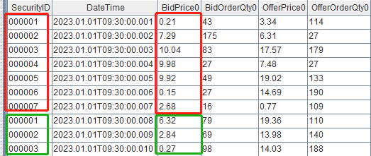
Create a reactive state engine and input this batch of data:
// Define input and output table schemas
colName = ["securityID","dateTime","preClosePx","openPx","highPx","lowPx","lastPx","totalVolumeTrade","totalValueTrade","instrumentStatus"] <- flatten(eachLeft(+, ["bidPrice","bidOrderQty","bidNumOrders"], string(0..9))) <- ("bidOrders"+string(0..49)) <- flatten(eachLeft(+, ["offerPrice","offerOrderQty","offerNumOrders"], string(0..9))) <- ("offerOrders"+string(0..49)) <- ["numTrades","iopv","totalBidQty","totalOfferQty","weightedAvgBidPx","weightedAvgOfferPx","totalBidNumber","totalOfferNumber","bidTradeMaxDuration","offerTradeMaxDuration","numBidOrders","numOfferOrders","withdrawBuyNumber","withdrawBuyAmount","withdrawBuyMoney","withdrawSellNumber","withdrawSellAmount","withdrawSellMoney","etfBuyNumber","etfBuyAmount","etfBuyMoney","etfSellNumber","etfSellAmount","etfSellMoney"]
colType = ["SYMBOL","TIMESTAMP","DOUBLE","DOUBLE","DOUBLE","DOUBLE","DOUBLE","INT","DOUBLE","SYMBOL"] <- take("DOUBLE", 10) <- take("INT", 70)<- take("DOUBLE", 10) <- take("INT", 70) <- ["INT","INT","INT","INT","DOUBLE","DOUBLE","INT","INT","INT","INT","INT","INT","INT","INT","DOUBLE","INT","INT","DOUBLE","INT","INT","INT","INT","INT","INT"]
inputTable = table(1:0, colName, colType)
resultTable = table(10000:0, ["securityID", "dateTime", "factor"], [SYMBOL, TIMESTAMP, DOUBLE])

// Create a reactive state engine
try{ dropStreamEngine("reactiveDemo")} catch(ex){ print(ex) }
rse = createReactiveStateEngine(name="reactiveDemo", metrics =metrics, dummyTable=inputTable, outputTable=resultTable, keyColumn="securityID")

// Input data
tableInsert(rse, testData.flip())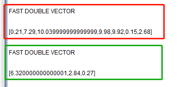
From the output, we can see that the function parameter bidPrice0 is a vector, and this batch of 10 records will be calculated in two passes (the first 7 records with different stock codes calculated once, and the last 3 records calculated once).
Therefore, when writing factor functions, we must pay attention to whether the functions we use support the data structure of the input parameters.
For example, now we want to add a conditional layer when calculating the weighted average price: if bidPrice0 > 0, perform the calculation; otherwise, return a default value:
def weightedAveragedPrice(bidPrice0, bidOrderQty0, offerPrice0, offerOrderQty0, default){
    if(bidPrice0 > 0){  return (bidPrice0*offerOrderQty0 + offerPrice0*bidOrderQty0) \ (offerOrderQty0+bidOrderQty0)}
    return default
}

metrics = <[dateTime, weightedAveragedPrice(bidPrice0, bidOrderQty0, offerPrice0, offerOrderQty0, 0.0)]>
If we directly pass the function weightedAveragedPrice to
the metrics parameter of the reactive state engine, the engine will
report an error: "A scalar object is expected. But the actual object is a
vector". This is because the if (condition){} else{}
control statement requires that condition must be a scalar, but the
bidPrice0 is a vector.
There are two solutions to this problem:
General Solution: Use higher-order traversal functions like
each/ loop to apply the function to
each element of the vector.
We can define a factorWeightedAveragedPrice function that
calls each to apply weightedAveragedPrice
to each element of bidPrice0, ensuring they are passed to the
function as scalars. Then specify the metrics parameter of the
reactive state engine as factorWeightedAveragedPrice for
calculation.
def factorWeightedAveragedPrice(bidPrice0, bidOrderQty0, offerPrice0, offerOrderQty0){
    return each(weightedAveragedPrice{default=0.0}, bidPrice0, bidOrderQty0, offerPrice0, offerOrderQty0)
}

metrics = <[dateTime, factorWeightedAveragedPrice(bidPrice0, bidOrderQty0, offerPrice0, offerOrderQty0)]>
Recommended Solution: For vector conditional control in this example,
we recommend using DolphinDB's built-in vector function iif
instead of if-else conditional statements:
def factorWeightedAveragedPrice(bidPrice0, bidOrderQty0, offerPrice0, offerOrderQty0){
    default = 0.0
    return iif(bidPrice0 > 0, (bidPrice0*offerOrderQty0 + offerPrice0*bidOrderQty0) \ (offerOrderQty0+bidOrderQty0), default)
}

metrics = <[dateTime, factorWeightedAveragedPrice(bidPrice0, bidOrderQty0, offerPrice0, offerOrderQty0)]>
3.2.2 Stateful Functions
A stateful function is a function that, in addition to using current data,
also relies on historical data during computation. For example, in Section
3.1.1, the price change factor pricePercentChange(price,
lag) requires not only the current price data but also
the historical price data for the past lag periods.
A state function must be declared using the @state
annotation.
Within a state function, only assignment statements, return
statements, and if-else statements are supported.
In if (condition) { ... } else { ... } statements, the
condition must be a scalar that does not depend on real-time
updating upstream table data. Continuing with the
pricePercentChange(price, lag) example: price
is a column from an upstream table that updates in real-time, while
lag is a separately specified window size. Therefore, a
condition like if (lag > 30) { ... } is valid, but
if (price > 0) { ... } is not allowed.
Alternatively, we can rewrite the logic using a vectorized function like
iif, as in iif(price > 0, ...,
...).
// price is a column from engine input table. So price > 0 is not a scalar as it updates in real-time
def pricePercentChange(price, lag){
    if(price>0){
        return price \ move(price, lag) - 1
    }else{
        return 0
    }
}

// lag is separately specified. So lag>30 returns a fixed scalar
@state
def pricePercentChange(price, lag){
    if(lag>30){
        return price \ move(price, lag) - 1
    }else{
        return price \ move(price, 30) - 1
    }
}
When defining a stateful function, we can use the row-based functions like
rowSum and rowMax, as well as
cumulative window functions like cumSum and
cumMax. However, aggregate functions like
sum and max are not allowed. For
aggregations in a stateful function, use the row-based functions, such as
rowSum. For example, to find the maximum of the current
price and the price from lag steps earlier (i.e.,
max(tradePrice[i], tradePrice[i-lag])), write the
factor like this:
// Factor implementation
@state
def maxPrice(price, lag){
    return rowMax([price, move(price, lag)])
}

// Define input and output table schemas
inputTable = table(1:0, `securityID`tradeTime`tradePrice`TradeQty`TradeAmount`BuyNo`SellNo`TradeBSFlag`TradeIndex`ChannelNo, [SYMBOL,DATETIME,DOUBLE,INT,DOUBLE,LONG,LONG,SYMBOL,INT,INT])
resultTable = table(10000:0, ["securityID", "tradeTime", "factor"], [SYMBOL, TIMESTAMP, DOUBLE])

// Create a reactive state engine
try{ dropStreamEngine("reactiveDemo")} catch(ex){ print(ex) }
metrics = <[tradeTime, maxPrice(tradePrice, 2)]>
rse = createReactiveStateEngine(name="reactiveDemo", metrics =metrics, dummyTable=inputTable, outputTable=resultTable, keyColumn="securityID")

// Input data
insert into rse values(`000155, 2020.01.01T09:30:00, 30.85, 100, 3085, 4951, 0, `B, 1, 1)
insert into rse values(`000155, 2020.01.01T09:30:01, 30.86, 100, 3086, 4951, 1, `B, 2, 1)
insert into rse values(`000155, 2020.01.01T09:30:02, 30.80, 200, 6160, 5501, 5600, `S, 3, 1)


// View results
select * from resultTable
/*
securityID tradeTime               factor
---------- ----------------------- ------------------
000155     2020.01.01T09:30:00.000 30.85
000155     2020.01.01T09:30:01.000 30.86
000155     2020.01.01T09:30:02.000 30.85
*/
Also keep in mind that any user-defined function that calls a stateful function must also be declared as a state function.
3.2.3 Separating Stateful/Stateless Computations
Reactive state engines support computations that combine both stateless and stateful functions. One of the most important steps for improving computational efficiency is separating stateful operations from stateless operations .
While certain stateless operations like rowSum can
technically be used inside a stateful function, it's generally not
recommended. Stateless functions are optimized for vectorized computation
and don’t need to maintain any internal state, making them much more
efficient. Therefore, instead of putting all your logic into a single
stateful function, it’s better to break out complex cross-sectional
(stateless) calculations into separate stateless functions. State functions
should mainly be reserved for custom logic that involves historical
data—such as sliding window operations, time-based windows, fill strategies,
or iterative computations. Below is an example to illustrate this.
3.2.3.1 Moving Average of Buy/Sell Pressure
Formulaic expressions
Step1. Calculate the buy/sell pressure indicator
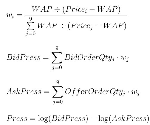
Step2. Compute the moving average of the buy/sell pressure over the past lag rows:
(press[i-lag+1]+…+press[i]) / lagCode implementation
Approach A. Implementing using a single stateful function (not recommended)
@state
def averagePress1(bidPrice0, bidPrice1, bidPrice2, bidPrice3, bidPrice4, bidPrice5, bidPrice6, bidPrice7, bidPrice8, bidPrice9, bidOrderQty0, bidOrderQty1, bidOrderQty2, bidOrderQty3, bidOrderQty4, bidOrderQty5, bidOrderQty6, bidOrderQty7, bidOrderQty8, bidOrderQty9, offerPrice0, offerPrice1, offerPrice2, offerPrice3, offerPrice4, offerPrice5, offerPrice6, offerPrice7, offerPrice8, offerPrice9, offerOrderQty0, offerOrderQty1, offerOrderQty2, offerOrderQty3, offerOrderQty4, offerOrderQty5, offerOrderQty6, offerOrderQty7, offerOrderQty8, offerOrderQty9, lag){
	bidPrice = fixedLengthArrayVector(bidPrice0, bidPrice1, bidPrice2, bidPrice3, bidPrice4, bidPrice5, bidPrice6, bidPrice7, bidPrice8, bidPrice9)
	bidOrderQty = fixedLengthArrayVector(bidOrderQty0, bidOrderQty1, bidOrderQty2, bidOrderQty3, bidOrderQty4, bidOrderQty5, bidOrderQty6, bidOrderQty7, bidOrderQty8, bidOrderQty9)
	offerPrice = fixedLengthArrayVector(offerPrice0, offerPrice1, offerPrice2, offerPrice3, offerPrice4, offerPrice5, offerPrice6, offerPrice7, offerPrice8, offerPrice9)
	offerOrderQty = fixedLengthArrayVector(offerOrderQty0, offerOrderQty1, offerOrderQty2, offerOrderQty3, offerOrderQty4, offerOrderQty5, offerOrderQty6, offerOrderQty7, offerOrderQty8, offerOrderQty9)
	wap = (bidPrice0*offerOrderQty0 + offerPrice0*bidOrderQty0) \ (offerOrderQty0+bidOrderQty0)
	bidPress = rowWavg(bidOrderQty, wap \ (bidPrice - wap))
	askPress = rowWavg(offerOrderQty, wap \ (offerPrice - wap))
	press = log(bidPress \ askPress)
	return mavg(press, lag, 1)
}
This approach is less efficient as it bundles all logic—stateless and stateful—into a single stateful function.
Approach B. Separating stateless and stateful logic (recommended)
def calPress(bidPrice0, bidPrice1, bidPrice2, bidPrice3, bidPrice4, bidPrice5, bidPrice6, bidPrice7, bidPrice8, bidPrice9, bidOrderQty0, bidOrderQty1, bidOrderQty2, bidOrderQty3, bidOrderQty4, bidOrderQty5, bidOrderQty6, bidOrderQty7, bidOrderQty8, bidOrderQty9, offerPrice0, offerPrice1, offerPrice2, offerPrice3, offerPrice4, offerPrice5, offerPrice6, offerPrice7, offerPrice8, offerPrice9, offerOrderQty0, offerOrderQty1, offerOrderQty2, offerOrderQty3, offerOrderQty4, offerOrderQty5, offerOrderQty6, offerOrderQty7, offerOrderQty8, offerOrderQty9){
	bidPrice = fixedLengthArrayVector(bidPrice0, bidPrice1, bidPrice2, bidPrice3, bidPrice4, bidPrice5, bidPrice6, bidPrice7, bidPrice8, bidPrice9)
	bidOrderQty = fixedLengthArrayVector(bidOrderQty0, bidOrderQty1, bidOrderQty2, bidOrderQty3, bidOrderQty4, bidOrderQty5, bidOrderQty6, bidOrderQty7, bidOrderQty8, bidOrderQty9)
	offerPrice = fixedLengthArrayVector(offerPrice0, offerPrice1, offerPrice2, offerPrice3, offerPrice4, offerPrice5, offerPrice6, offerPrice7, offerPrice8, offerPrice9)
	offerOrderQty = fixedLengthArrayVector(offerOrderQty0, offerOrderQty1, offerOrderQty2, offerOrderQty3, offerOrderQty4, offerOrderQty5, offerOrderQty6, offerOrderQty7, offerOrderQty8, offerOrderQty9)
	wap = (bidPrice0*offerOrderQty0 + offerPrice0*bidOrderQty0) \ (offerOrderQty0+bidOrderQty0)
	bidPress = rowWavg(bidOrderQty, wap \ (bidPrice - wap))
	askPress = rowWavg(offerOrderQty, wap \ (offerPrice - wap))
	press = log(bidPress \ askPress)
	return press
}

@state
def averagePress2(bidPrice0, bidPrice1, bidPrice2, bidPrice3, bidPrice4, bidPrice5, bidPrice6, bidPrice7, bidPrice8, bidPrice9, bidOrderQty0, bidOrderQty1, bidOrderQty2, bidOrderQty3, bidOrderQty4, bidOrderQty5, bidOrderQty6, bidOrderQty7, bidOrderQty8, bidOrderQty9, offerPrice0, offerPrice1, offerPrice2, offerPrice3, offerPrice4, offerPrice5, offerPrice6, offerPrice7, offerPrice8, offerPrice9, offerOrderQty0, offerOrderQty1, offerOrderQty2, offerOrderQty3, offerOrderQty4, offerOrderQty5, offerOrderQty6, offerOrderQty7, offerOrderQty8, offerOrderQty9, lag){
	press = calPress(bidPrice0, bidPrice1, bidPrice2, bidPrice3, bidPrice4, bidPrice5, bidPrice6, bidPrice7, bidPrice8, bidPrice9, bidOrderQty0, bidOrderQty1, bidOrderQty2, bidOrderQty3, bidOrderQty4, bidOrderQty5, bidOrderQty6, bidOrderQty7, bidOrderQty8, bidOrderQty9, offerPrice0, offerPrice1, offerPrice2, offerPrice3, offerPrice4, offerPrice5, offerPrice6, offerPrice7, offerPrice8, offerPrice9, offerOrderQty0, offerOrderQty1, offerOrderQty2, offerOrderQty3, offerOrderQty4, offerOrderQty5, offerOrderQty6, offerOrderQty7, offerOrderQty8, offerOrderQty9)
	return mavg(press, lag, 1)
}
3.2.3.2 Performance Comparison
DolphinDB Server Version: 2.00.9.2 (2023.03.10 JIT)
Dataset: Level-2 snapshot data for 100 stocks, one trading day; 372,208 rows × 194 columns (319MB)
Method: Measure the total time from the start of data ingestion to
completion of factor calculations using the timer
function.
Result:
| Implementation Approach | Execution Time (ms) |
|---|---|
| All logic in one state function | 1492.224 |
| Stateless + state function split | 577.651 |
Test script:
// Import test data
csvPath = "/path/to/testdata/"
colName = ["securityID","dateTime","preClosePx","openPx","highPx","lowPx","lastPx","totalVolumeTrade","totalValueTrade","instrumentStatus"] <- flatten(eachLeft(+, ["bidPrice","bidOrderQty","bidNumOrders"], string(0..9))) <- ("bidOrders"+string(0..49)) <- flatten(eachLeft(+, ["offerPrice","offerOrderQty","offerNumOrders"], string(0..9))) <- ("offerOrders"+string(0..49)) <- ["numTrades","iopv","totalBidQty","totalOfferQty","weightedAvgBidPx","weightedAvgOfferPx","totalBidNumber","totalOfferNumber","bidTradeMaxDuration","offerTradeMaxDuration","numBidOrders","numOfferOrders","withdrawBuyNumber","withdrawBuyAmount","withdrawBuyMoney","withdrawSellNumber","withdrawSellAmount","withdrawSellMoney","etfBuyNumber","etfBuyAmount","etfBuyMoney","etfSellNumber","etfSellAmount","etfSellMoney"]
colType = ["SYMBOL","TIMESTAMP","DOUBLE","DOUBLE","DOUBLE","DOUBLE","DOUBLE","INT","DOUBLE","SYMBOL"] <- take("DOUBLE", 10) <- take("INT", 70)<- take("DOUBLE", 10) <- take("INT", 70) <- ["INT","INT","INT","INT","DOUBLE","DOUBLE","INT","INT","INT","INT","INT","INT","INT","INT","DOUBLE","INT","INT","DOUBLE","INT","INT","INT","INT","INT","INT"]
data = select * from loadText(csvPath + "snapshot_100stocks_multi.csv", schema=table(colName, colType)) order by dateTime

// Define input and output schemas
inputTable = table(1:0, colName, colType)
resultTable1 = table(10000:0, ["securityID", "dateTime", "factor"], [SYMBOL, TIMESTAMP, DOUBLE])
resultTable2 = table(10000:0, ["securityID", "dateTime", "factor"], [SYMBOL, TIMESTAMP, DOUBLE])

// Create a reactive state engine
// All logic in one state function
try{ dropStreamEngine("reactiveDemo1")} catch(ex){ print(ex) }
metrics1 = <[dateTime, averagePress1(bidPrice0, bidPrice1, bidPrice2, bidPrice3, bidPrice4, bidPrice5, bidPrice6, bidPrice7, bidPrice8, bidPrice9, bidOrderQty0, bidOrderQty1, bidOrderQty2, bidOrderQty3, bidOrderQty4, bidOrderQty5, bidOrderQty6, bidOrderQty7, bidOrderQty8, bidOrderQty9, offerPrice0, offerPrice1, offerPrice2, offerPrice3, offerPrice4, offerPrice5, offerPrice6, offerPrice7, offerPrice8, offerPrice9, offerOrderQty0, offerOrderQty1, offerOrderQty2, offerOrderQty3, offerOrderQty4, offerOrderQty5, offerOrderQty6, offerOrderQty7, offerOrderQty8, offerOrderQty9, 60)]>
rse1 = createReactiveStateEngine(name="reactiveDemo1", metrics =metrics1, dummyTable=inputTable, outputTable=resultTable1, keyColumn="securityID")
// Stateless + state function split
try{ dropStreamEngine("reactiveDemo2")} catch(ex){ print(ex) }
metrics2 = <[dateTime, averagePress2(bidPrice0, bidPrice1, bidPrice2, bidPrice3, bidPrice4, bidPrice5, bidPrice6, bidPrice7, bidPrice8, bidPrice9, bidOrderQty0, bidOrderQty1, bidOrderQty2, bidOrderQty3, bidOrderQty4, bidOrderQty5, bidOrderQty6, bidOrderQty7, bidOrderQty8, bidOrderQty9, offerPrice0, offerPrice1, offerPrice2, offerPrice3, offerPrice4, offerPrice5, offerPrice6, offerPrice7, offerPrice8, offerPrice9, offerOrderQty0, offerOrderQty1, offerOrderQty2, offerOrderQty3, offerOrderQty4, offerOrderQty5, offerOrderQty6, offerOrderQty7, offerOrderQty8, offerOrderQty9, 60)]>
rse2 = createReactiveStateEngine(name="reactiveDemo2", metrics =metrics2, dummyTable=inputTable, outputTable=resultTable2, keyColumn="securityID")

// Insert data
timer rse1.append!(data)
timer rse2.append!(data)

// Verify results
each(eqObj, resultTable1.values(), resultTable2.values()).all()
3.2.3.3 Key Considerations
(1) Due to internal handling by the reactive state engine, not all data types can be passed between stateless and stateful functions. Specifically:
- Supported: Scalars, vectors, and array vectors
- Not Supported: Tuples (ANY VECTOR type)
The following example explains this by printing the data types and values
of the parameters passed from a stateful function to a stateless
function using print.
// Factor implementation
def typeTestNonStateFunc(scalar, vector, arrayVector, anyVector){
	print("---------------------------------------")
	print(typestr(scalar))
	print(scalar)
	print(typestr(vector))
	print(vector)
	print(typestr(arrayVector))
	print(arrayVector)
	print(typestr(anyVector))
	print(anyVector)
	return fixedLengthArrayVector(rowSum(arrayVector), rowAvg(arrayVector))
}

@state
def typeTestStateFunc(price1, price2, price3, lag){
	scalar = lag
	vector = price1
	arrayVector = fixedLengthArrayVector(price1, price2, price3)
	anyVector = [price1, price2, price3]
	res = typeTestNonStateFunc(scalar, vector, arrayVector, anyVector)
	sumRes = res[0]
	avgRes = res[1]
	return sumRes, avgRes, res, anyVector
}
In this example, lag is a constant value specified separately, and
price1, price2, and price3 are three columns
from the upstream input table. The function
fixedLengthArrayVector is used to combine multiple
vectors into an array vector, and [price1, price2,
price3] forms a tuple.
// Define input and output table schemas
inputTable = table(1:0, `securityID`tradeTime`price1`price2`price3, [SYMBOL,DATETIME,DOUBLE,DOUBLE,DOUBLE])
resultTable = table(10000:0, ["securityID", "tradeTime", "sum", "avg", "sum_avg", "anyVector"], [SYMBOL, TIMESTAMP, DOUBLE, DOUBLE, DOUBLE[], DOUBLE[]])

// Create the reactive state engine
try{ dropStreamEngine("reactiveDemo")} catch(ex){ print(ex) }
metrics = <[tradeTime, typeTestStateFunc(price1, price2, price3, 10) as `sum`avg`sum_avg`anyVector]>
rse = createReactiveStateEngine(name="reactiveDemo", metrics=metrics, dummyTable=inputTable, outputTable=resultTable, keyColumn="securityID")

// Input data
insert into rse values(`000155, 2020.01.01T09:30:00, 30.81, 30.82, 30.83)
insert into rse values(`000155, 2020.01.01T09:30:01, 30.86, 30.87, 30.88)
insert into rse values(`000155, 2020.01.01T09:30:02, 30.80, 30.81, 30.82)

// View the results
select * from resultTable
/*
securityID tradeTime               sum    avg    sum_avg                 anyVector
---------- ----------------------- ------ ------ ----------------------- ---------
000155     2020.01.01T09:30:00.000 92.46  30.82  [92.46,30.82]           [00F]
000155     2020.01.01T09:30:01.000 92.61  30.87  [92.61,30.87]           [00F]
000155     2020.01.01T09:30:02.000 92.43  30.81  [92.43,30.81]           [00F]
*/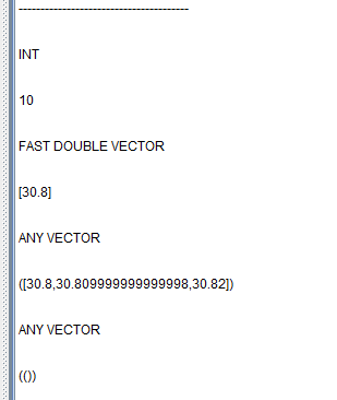
We can see that the tuple column is NULL.
(2) When calling a user-defined function inside a stateful function, it
is not supported to receive multiple return values using multiple
variables (i.e., the syntax a, b = foo(...) is not
allowed). If a stateless function needs to return multiple values, they
should be assembled into an array vector using
fixedLengthArrayVector and returned as a single
value. Within the stateful function, hold the result using one variable
and then access individual values via indexing (e.g.,
res[0] from example above.)
(3) Once the data has been assembled into an array vector, aggregation in
each row must use the row-based functions or the byRow
higher-order function. Refer to the example above, where the sum of
three prices is calculated using rowSum, and the
average is calculated using rowAvg.
3.3 if-else Statements
Both stateless and stateful functions support the use of if-else
statements. As mentioned earlier, in stateless functions, the condition in the
if-else statement must be a scalar. For stateful functions,
the condition must also be a scalar, and one that is independent of the upstream
table. Typically, you can use the built-in iif function as a
replacement for if-else. For examples, refer to section 3.2.1
for stateless functions and section 3.2.2 for stateful functions.
The iif(cond, trueResult, falseResult) function evaluates
both trueResult and falseResult regardless of the condition,
and then returns either trueResult or falseResult based on the
condition cond. Therefore, expressions of both trueResult and
falseResult must be valid and executable for all possible input
scenarios. For example, y = iif(size(x) > 0, sum(x), 0.0)
calculates both expressions: if x = [], although the
condition size(x) > 0 is false and should return 0.0,
iif will still evaluate both expressions. As a result,
sum(x) will be computed, which causes an error because
sum(x) does not accept an empty vector. In this case,
it is better to use an if-else statement:
if(size(x) > 0) { y = sum(x) } else { y = 0 }.
3.4. Historical Data Access (Windowing and Iteration)
DolphinDB provides a rich set of built-in functions to help users perform various
stateful calculations involving historical data. For example, sliding window
functions, time-based sliding window functions, cumulative window functions, and
filling functions like ffill are available.
In addition, movingWindowData and
tmovingWindowData directly return an array vector where
each row consists of the elements of a window sliding over the input data. This
makes it easier for users to implement custom calculations.
Although stateful functions do not support recursive calls, DolphinDB offers
functions such as conditionalIterate,
stateIterate, genericStateIterate, and
genericTStateIterate to support iteration logic and more
complex processing of historical data.
The following is an example of how to implement a complex factor with custom logic.
Formulaic expressions
Step 1: Based on snapshot data, calculate weighted averages of first-level bid/ask prices and volumes by applying specified weights over the most recent lag records:
bidPrice = bidPrice0[i-lag+1]*weight[0] + … + bidPrice0[i]*weight[lag-1]
askPrice = offerPrice0[i-lag+1]*weight[0] + … + offerPrice0[i]*weight[lag-1]
bidVolume = bidOrderQty0[i-lag+1]*weight[0] + … + bidOrderQty0[i]*weight[lag-1]
askVolume = offerOrderQty0[i-lag+1]*weight[0] + … + offerOrderQty0[i]*weight[lag-1]
Step 2: Calculate the moving average weighted price (maWAP) using the results from Step 1.
Step 3: The factor result is the weighted average of the previous lag-1 factor values and the current maWAP:
w[i] = bidVolume[i-lag]/askVolume[i-lag]
factor[i] = (factor[i-lag+1]*w[i-lag+1] + ... + factor[i-1]*w[i-1] + maWAP[i]*w[i]) / (w[i-lag+1] + ... + w[i])
Code implementation
defg myWavg(x){
	weight = 1..size(x)
	return wavg(x, weight)
}

def iterateFunc(historyFactors, currentValue, weight){
	return wavg(historyFactors join currentValue, weight)
}

@state
def myFactor(bidPrice0, bidOrderQty0, offerPrice0, offerOrderQty0, lag){
	// Step 1: Use moving
    bidPrice, askPrice, bidVolume, askVolume = moving(myWavg, bidPrice0, lag, 1), moving(myWavg, offerPrice0, lag, 1), moving(myWavg, bidOrderQty0, lag, 1), moving(myWavg, offerOrderQty0, lag, 1)

    // Step 2: Use mavg
    wap = (bidPrice*askVolume + askPrice*bidVolume) \ (bidVolume + askVolume)
    maWap = mavg(wap, lag, 1)

    // Step 3: Use movingWindowData
    w = movingWindowData(bidVolume \ askVolume, lag)

    // Use genericStateIterate
    factorValue = genericStateIterate(X=[maWap, w], initial=maWap, window=lag-1, func=iterateFunc)
    return factorValue
}
Stream processing script
// Define input and output schemas
colName = ["securityID", "dateTime", "preClosePx", "openPx", "highPx", "lowPx", "lastPx", "totalVolumeTrade", "totalValueTrade", "instrumentStatus"]
colType = ["SYMBOL", "TIMESTAMP", "DOUBLE", "DOUBLE", "DOUBLE", "DOUBLE", "DOUBLE", "INT", "DOUBLE", "SYMBOL"]
inputTable = table(1:0, colName, colType)
resultTable = table(10000:0, ["securityID", "dateTime", "factor"], [SYMBOL, TIMESTAMP, DOUBLE])

// Create the reactive state engine
try{ dropStreamEngine("reactiveDemo")} catch(ex){ print(ex) }
metrics = <[dateTime, myFactor(bidPrice0, bidOrderQty0, offerPrice0, offerOrderQty0, 3)]>
rse = createReactiveStateEngine(name="reactiveDemo", metrics=metrics, dummyTable=inputTable, outputTable=resultTable, keyColumn="securityID")

// Insert data
tableInsert(rse, {"securityID":"000001", "dateTime":2023.01.01T09:30:00.000, "bidPrice0":19.98, "bidOrderQty0":100, "offerPrice0":19.99, "offerOrderQty0":120})
tableInsert(rse, {"securityID":"000001", "dateTime":2023.01.01T09:30:03.000, "bidPrice0":19.95, "bidOrderQty0":130, "offerPrice0":19.93, "offerOrderQty0":120})
tableInsert(rse, {"securityID":"000001", "dateTime":2023.01.01T09:30:06.000, "bidPrice0":19.97, "bidOrderQty0":120, "offerPrice0":19.98, "offerOrderQty0":130})
tableInsert(rse, {"securityID":"000001", "dateTime":2023.01.01T09:30:09.000, "bidPrice0":20.00, "bidOrderQty0":130, "offerPrice0":19.97, "offerOrderQty0":140})

// View the results
select * from resultTable
/*
securityID dateTime                factor
---------- ----------------------- ------------------
000001     2023.01.01T09:30:00.000 19.9845
000001     2023.01.01T09:30:03.000 19.9698
000001     2023.01.01T09:30:06.000 19.9736
000001     2023.01.01T09:30:09.000 19.9694
*/- In the higher-order function
moving(func, ...), func is an aggregate function that must be declared using thedefgkeyword. - Stateful functions do not support recursive calls. So, when we need to
access historical factor values (such as using the previous value when
the current calculation is empty), it becomes challenging to express
this logic. To address this, DolphinDB provides functions like
conditionalIterate. However, functions likeconditionalIteratedon't store the final return value of the factor function, but instead store the results calculated up to the current line of code execution. Therefore, functions likeconditionalIterateshould be placed at the end of the factor function to ensure the correct historical data is used for calculations.
Here is an example to illustrate this behavior:
@state
def iterateTestFunc(tradePrice):{
    // Calculate the change in trade price
    change = tradePrice \ prev(tradePrice) - 1
    // If the result is null, fill it with the previous non-null factor value
    factor = conditionalIterate(change != NULL, change, cumlastNot)
    // Return factor + 1 as the final factor value
    return factor + 1
}
Create the reactive state engine and insert some data:
// Define input and output schemas
inputTable = table(1:0, `securityID`tradeTime`tradePrice`tradeQty`tradeAmount`buyNo`sellNo`tradeBSFlag`tradeIndex`channelNo, [SYMBOL,DATETIME,DOUBLE,INT,DOUBLE,LONG,LONG,SYMBOL,INT,INT])
resultTable = table(10000:0, ["securityID", "tradeTime", "factor"], [SYMBOL, TIMESTAMP, DOUBLE])

// Create the reactive state engine
try{ dropStreamEngine("reactiveDemo")} catch(ex){ print(ex) }
metrics = <[tradeTime, iterateTestFunc(tradePrice)]>
rse = createReactiveStateEngine(name="reactiveDemo", metrics=metrics, dummyTable=inputTable, outputTable=resultTable, keyColumn="securityID")

// Insert data
insert into rse values(`000155, 2020.01.01T09:30:00, 30.85, 100, 3085, 4951, 0, `B, 1, 1)
insert into rse values(`000155, 2020.01.01T09:30:01, 30.86, 100, 3086, 4951, 1, `B, 2, 1)
insert into rse values(`000155, 2020.01.01T09:30:02, NULL, NULL, NULL, NULL, NULL, NULL, NULL, NULL)
insert into rse values(`000155, 2020.01.01T09:30:03, 30.80, 200, 6160, 5501, 5600, `S, 3, 1)

// View the results
select * from resultTable
/*
securityID tradeTime               factor
---------- ----------------------- ----------------
000155     2020.01.01T09:30:00.000
000155     2020.01.01T09:30:01.000 1.0003
000155     2020.01.01T09:30:02.000 1.0003
000155     2020.01.01T09:30:03.000 1.0003
*/| tradeTime | tradePrice | change | cumlastNot | factor=conditionalIterate(…) | iterateTestFunc(tradePrice) |
|---|---|---|---|---|---|
| 2020.01.01T09:30:00 | 30.85 | NULL | NULL | NULL | NULL |
| 2020.01.01T09:30:01 | 30.86 | 0.0003 | NULL | 0.0003 | 1.0003 |
| 2020.01.01T09:30:02 | NULL | NULL | 0.0003 | 0.0003 | 1.0003 |
| 2020.01.01T09:30:03 | 30.80 | NULL | 0.0003 | 0.0003 | 1.0003 |
As we can see from the table above, in the line factor =
conditionalIterate(change != NULL, change, cumlastNot), the
cumlastNot function is not looking for the previous
non-null value of the factor function iterateTestFunc, but
rather the previous non-null value of “factor”. The final step in the factor
function, factor+1, is not recorded by the
conditionalIterate function.
To perform operations on historical factor values, consider using functions like
stateIterate or genericStateIterate. For
example, the above example can be rewritten as:
// Currently window >= 2 is required, so we need window=2 even to look back at the previous value
def processFunc(historyFactor, change){
    lastFactor = last(historyFactor)
    factor = iif(change != NULL, change, lastFactor)
    return factor+1
}

@state
def iterateTestFunc(tradePrice){
    // Calculate the change in trade price
    change = tradePrice \ prev(tradePrice) - 1
    // If the result is null, fill it with the previous factor value, and return factor+1 as the final value
    factor = genericStateIterate(X=[change], initial=change, window=2, func=processFunc)
    return factor
}

// When window=1 is supported in the future, the following code can be used instead
/*
def processFunc(lastFactor, change){
    factor = iif(change != NULL, change, lastFactor)
    return factor+1
}

@state
def iterateTestFunc(tradePrice){
    // Calculate the change in trade price
    change = tradePrice \ prev(tradePrice) - 1
    // If the result is null, fill it with the previous factor value, and return factor+1 as the final value
    factor = genericStateIterate(X=[change], initial=change, window=1, func=processFunc)
    return factor
}
*/| tradeTime | tradePrice | change | lastFactor | factor=iif(..) | iterateTestFunc(tradePrice) |
|---|---|---|---|---|---|
| 2020.01.01T09:30:00 | 30.85 | NULL | NULL | NULL | NULL |
| 2020.01.01T09:30:01 | 30.86 | 0.0003 | NULL | 0.0003 | 1.0003 |
| 2020.01.01T09:30:02 | NULL | NULL | 1.0003 | 1.0003 | 2.0003 |
| 2020.01.01T09:30:03 | 30.80 | NULL | 2.0003 | 2.0003 | 3.0003 |
3.5 Loops
Stateful functions do not allow for or while
statements, but they support loop logic through functions such as
each and loop.
The following example demonstrates how to implement loop logic within a reactive state engine.
Factor calculation logic (in Python)
def _bid_withdraws_volume(l, n, levels=10):
    withdraws = 0
    for price_index in range(0,4*levels, 4):
        now_p = n[price_index]
        for price_last_index in range(0,4*levels,4):
            if l[price_last_index] == now_p:
                withdraws -= min(n[price_index+1] - l[price_last_index + 1], 0)
    return withdraws

def bid_withdraws(depth, trade):
    ob_values = depth.values
    flows = np.zeros(len(ob_values))
    for i in range(1, len(ob_values)):
        flows[i] = _bid_withdraws_volume(ob_values[i-1], ob_values[i])
    return pd.Series(flows)
In the script above, there are two nested loops in this factor. The inner loop
can be converted into a vectorized calculation, while the outer loop can be
implemented using the each function.
DolphinDB code implementation
// For the inner loop
def withdrawsVolumeTmp(lastPrices, lastVolumes, nowPrice, nowVolume):
    withdraws = lastVolumes[lastPrices == nowPrice] - nowVolume
    return sum(withdraws * (withdraws > 0))

// For the outer loop
defg withdrawsVolume(prices, Volumes):
    lastPrices, nowPrices = prices[0], prices[1]
    lastVolumes, nowVolumes = Volumes[0], Volumes[1]

    withdraws = each(withdrawsVolumeTmp{lastPrices, lastVolumes}, nowPrices, nowVolumes)
    return sum(withdraws)

@state
def bidWithdrawsVolume(bidPrice0, bidPrice1, bidPrice2, bidPrice3, bidPrice4, bidPrice5, bidPrice6, bidPrice7, bidPrice8, bidPrice9,bidOrderQty0, bidOrderQty1, bidOrderQty2, bidOrderQty3, bidOrderQty4, bidOrderQty5, bidOrderQty6, bidOrderQty7, bidOrderQty8, bidOrderQty9, levels=10){
	bidPrice = fixedLengthArrayVector(bidPrice0, bidPrice1, bidPrice2, bidPrice3, bidPrice4, bidPrice5, bidPrice6, bidPrice7, bidPrice8, bidPrice9)
	bidOrderQty = fixedLengthArrayVector(bidOrderQty0, bidOrderQty1, bidOrderQty2, bidOrderQty3, bidOrderQty4, bidOrderQty5, bidOrderQty6, bidOrderQty7, bidOrderQty8, bidOrderQty9)
	return moving(withdrawsVolume, [bidPrice[0:levels], bidOrderQty[0:levels]], 2)
}
Stream processing script
// Define input and output schemas
colName = ["securityID", "dateTime", "preClosePx", "openPx", "highPx", "lowPx", "lastPx", "totalVolumeTrade", "totalValueTrade", "instrumentStatus"]
colType = ["SYMBOL", "TIMESTAMP", "DOUBLE", "DOUBLE", "DOUBLE", "DOUBLE", "DOUBLE", "INT", "DOUBLE", "SYMBOL"]
inputTable = table(1:0, colName, colType)
resultTable = table(10000:0, ["securityID", "dateTime", "factor"], [SYMBOL, TIMESTAMP, DOUBLE])

// Create the reactive state engine
try { dropStreamEngine("reactiveDemo") } catch (ex) { print(ex) }
metrics = <[dateTime, bidWithdrawsVolume(bidPrice0, bidPrice1, bidPrice2, bidPrice3, bidPrice4, bidPrice5, bidPrice6, bidPrice7, bidPrice8, bidPrice9,
                                       bidOrderQty0, bidOrderQty1, bidOrderQty2, bidOrderQty3, bidOrderQty4, bidOrderQty5, bidOrderQty6, bidOrderQty7,
                                       bidOrderQty8, bidOrderQty9, levels=3)]>
rse = createReactiveStateEngine(name="reactiveDemo", metrics=metrics, dummyTable=inputTable, outputTable=resultTable, keyColumn="securityID")

// Generate test data
setRandomSeed(9)
n = 5
securityID = take(`000001, n)
dateTime = 2023.01.01T09:30:00.000 + 1..n*3*1000
bidPrice0 = rand(10, n) \ 100 + 19.5
bidPrice1, bidPrice2 = bidPrice0 + 0.01, bidPrice0 + 0.02
bidOrderQty0, bidOrderQty1, bidOrderQty2 = rand(200, n), rand(200, n), rand(200, n)
offerPrice0 = rand(10, n) \ 100 + 19.5
offerPrice1, offerPrice2 = offerPrice0 + 0.01, offerPrice0 + 0.02
offerOrderQty0, offerOrderQty1, offerOrderQty2 = rand(200, n), rand(200, n), rand(200, n)
testdata = table(securityID, dateTime, bidPrice0, bidPrice1, bidPrice2, bidOrderQty0, bidOrderQty1, bidOrderQty2, offerPrice0, offerPrice1, offerPrice2, offerOrderQty0, offerOrderQty1, offerOrderQty2)

// Insert data
tableInsert(rse, testdata.flip())

// View the results
select * from resultTable
/*
securityID dateTime                factor
---------- ----------------------- ------
000001     2023.01.01T09:30:03.000
000001     2023.01.01T09:30:06.000
000001     2023.01.01T09:30:09.000 0
000001     2023.01.01T09:30:12.000 36
000001     2023.01.01T09:30:15.000 26
*/
4. Optimizing High-Frequency Factor Streaming
4.1. Array Vector
Array vectors are a special type of vector designed to store variable-length arrays, which can significantly simplify queries and calculations in some scenarios. When columns contain repetitive data, consolidating them into a single array vector column improves data compression and accelerates query performance. Array vectors support binary operations with scalars, vectors, or other array vectors, enabling vectorization of factor calculation logic.
High-frequency factors based on Level 2 market data typically involve operations
across the 10 best prices and their corresponding volumes. In previous
implementations, we often had to use the fixedLengthArrayVector
function to consolidate price and volume columns into array vector columns for
vectorized calculations. By directly storing multiple levels of price and volume
data as array vectors from the start, we can simplify factor function
definitions and improve calculation performance.
Consider using array vectors in the implementation of the "moving average buy-sell pressure" (from section 3.2.3.1) factor:
def pressArrayVector(bidPrice, bidOrderQty, offerPrice, offerOrderQty){
	wap = (bidPrice[0]*offerOrderQty[0] + offerPrice[0]*bidOrderQty[0]) \ (offerOrderQty[0]+bidOrderQty[0])
	bidPress = rowWavg(bidOrderQty, wap \ (bidPrice - wap))
	askPress = rowWavg(offerOrderQty, wap \ (offerPrice - wap))
	press = log(bidPress \ askPress)
	return press
}

@state
def averagePress3(bidPrice, bidOrderQty, offerPrice, offerOrderQty, lag){
	press = pressArrayVector(bidPrice, bidOrderQty, offerPrice, offerOrderQty)
	return mavg(press, lag, 1)
}- For row-wise calculations on array vectors, use row-based functions or
the
byRowhigher-order function. For example,rowSum(bidPrice)calculates the sum of the 10 best prices at each time point. - Data appended to an array vector column must have the same data type.
For example, if the engine's input schema (specified by
dummyTable) defines an array vector column as
INT[]type, the corresponding column in the inserting data must also beINT[]. - Take into account the computational cost of slicing and indexing operations on array vectors. If your factor requires complex operations across multiple or all 10 price/volume levels, using a single array vector column improves performance. However, if your factor only operates on individual levels (like only the best bid price), storing prices in separate columns may be more efficient.
4.2. Just-In-Time (JIT) Compilation
DolphinDB is implemented in C++ at its core, and a single function call in a script is translated into multiple virtual function calls within C++. When vectorization cannot be used, the interpretation cost can be relatively high.
The Just-In-Time (JIT) compilation feature in DolphinDB translates code into
machine code at runtime, significantly improving the execution speed of
statements like for loops, while loops, and
if-else structures. This is especially useful in scenarios
where vectorization cannot be applied but high performance is critical, such as
high-frequency factor calculations and real-time stream data processing. For a
detailed guide on using JIT, refer to the Just-in-time (JIT) Compilation. Note that this feature requires a
DolphinDB JIT server.
This section focuses on the considerations when writing JIT-enabled factor expressions in the reactive state engine.
A factor in the reactive state engine is typically a combination of stateful and stateless functions. The main difference between JIT-enabled factors and non-JIT factors lies in the stateless functions; there is no difference in how stateful functions are handled.
Key Differences:
- JIT functions require the
@jitannotation. - Stateless functions in the standard (non-JIT) DolphinDB server have no usage
restrictions, while the DolphinDB JIT server only supports certain
functions. Functions not supported in JIT require users to manually
implement them using techniques like formula expansion,
for/whileloops, andif-elsestatements. Below are some examples:Example 1. Using formula expansion to implement the
sumfunction when calculating the total of the top 10 bid prices:Formulaic expression:
bidPrice0*bidOrderQty0 + … +
                            bidPrice9*bidOrderQty9
Code implementation
@jit
def calAmount(bidPrice0, bidPrice1, bidPrice2, bidPrice3, bidPrice4, bidPrice5, bidPrice6, bidPrice7, bidPrice8, bidPrice9, bidOrderQty0, bidOrderQty1, bidOrderQty2, bidOrderQty3, bidOrderQty4, bidOrderQty5, bidOrderQty6, bidOrderQty7, bidOrderQty8, bidOrderQty9){
	return bidPrice0*bidOrderQty0+bidPrice1*bidOrderQty1+bidPrice2*bidOrderQty2+bidPrice3*bidOrderQty3+bidPrice4*bidOrderQty4+bidPrice5*bidOrderQty5+bidPrice6*bidOrderQty6+bidPrice7*bidOrderQty7+bidPrice8*bidOrderQty8+bidPrice9*bidOrderQty9
}
Example 2. Using a
forloop andif-elsestatement to implement themaxfunction when calculating the maximum total of the top 10 bid prices.Formulaic expression:
max(bidPrice0*bidOrderQty0, …,
                                bidPrice9*bidOrderQty9)
Code implementation
@jit def calAmountMax(bidPrice0, bidPrice1, bidPrice2, bidPrice3, bidPrice4, bidPrice5, bidPrice6, bidPrice7, bidPrice8, bidPrice9, bidOrderQty0, bidOrderQty1, bidOrderQty2, bidOrderQty3, bidOrderQty4, bidOrderQty5, bidOrderQty6, bidOrderQty7, bidOrderQty8, bidOrderQty9){ amount = [bidPrice0*bidOrderQty0, bidPrice1*bidOrderQty1, bidPrice2*bidOrderQty2, bidPrice3*bidOrderQty3, bidPrice4*bidOrderQty4, bidPrice5*bidOrderQty5, bidPrice6*bidOrderQty6, bidPrice7*bidOrderQty7, bidPrice8*bidOrderQty8, bidPrice9*bidOrderQty9] maxRes = -1.0 for(i in 0:10){ if(amount[i] > maxRes) maxRes = amount[i] } return maxRes }Note:When assigning initial or default values to variables, ensure the data type consistency before and after initialization. For instance, if the maxRes variable is of type DOUBLE, the initial value should bemaxRes=-1.0, notmaxRes=-1. - In the standard (non-JIT) DolphinDB server, the input to a stateless
function is treated as a vector (refer to section 3.2.1 "Stateless
Calculations" for details). In the JIT server, inputs are scalars, so no
extra processing (such as using
eachorloop) is required.Using the example from section 3.2.1 "Stateless Calculations", we can directly add the
@jitannotation outside theweightedAveragedPricefunction without needing additionaleachprocessing inside thefactorWeightedAveragedPricefunction:// Factor implementation @jit def weightedAveragedPrice(bidPrice0, bidOrderQty0, offerPrice0, offerOrderQty0, default){ if(bidPrice0 > 0){ return (bidPrice0*offerOrderQty0 + offerPrice0*bidOrderQty0) \ (offerOrderQty0+bidOrderQty0)} return default } metrics = <[dateTime, weightedAveragedPrice(bidPrice0, bidOrderQty0, offerPrice0, offerOrderQty0, 0.0)]> - In the JIT version, we can access specific elements of a vector using
vector[index]. However, the index can only be a scalar (e.g.,index = 0) or a vector (e.g.,index = 0..5). It cannot be a data pair (e.g.,index = 0:5). - In the JIT version, default parameters cannot be set in function
definitions. For example,
def foo(x, y){}is allowed, butdef foo(x, y=1){}is not.
4.3. Performance Testing
DolphinDB Server Version: 2.00.9.2 (2023.03.10 JIT)
Dataset: Level-2 snapshot data on a specific day (372,208 records)
Method: Measure the total time from the start of data ingestion to
completion of factor calculations using the timer function.
Factor:
After filtering out empty price levels from the top 10 bid and ask levels, we calculate the moving average of buy/sell pressure (See section 3.2.3.1 for the formulaic expression).
Results:
| Implementation Approach | Execution Time (ms) |
|---|---|
| Multi-column (per price level) | 6368.81 |
| Array vector columns | 3727.03 |
| Multi-column (per price level) + JIT | 771.13 |
| Array vector columns + JIT | 458.56 |
Code Implementations
Multi-column implementation
def calPress(bidPrice0, bidPrice1, bidPrice2, bidPrice3, bidPrice4, bidPrice5, bidPrice6, bidPrice7, bidPrice8, bidPrice9, bidOrderQty0, bidOrderQty1, bidOrderQty2, bidOrderQty3, bidOrderQty4, bidOrderQty5, bidOrderQty6, bidOrderQty7, bidOrderQty8, bidOrderQty9, offerPrice0, offerPrice1, offerPrice2, offerPrice3, offerPrice4, offerPrice5, offerPrice6, offerPrice7, offerPrice8, offerPrice9, offerOrderQty0, offerOrderQty1, offerOrderQty2, offerOrderQty3, offerOrderQty4, offerOrderQty5, offerOrderQty6, offerOrderQty7, offerOrderQty8, offerOrderQty9){
	bidPrice = [bidPrice0, bidPrice1, bidPrice2, bidPrice3, bidPrice4, bidPrice5, bidPrice6, bidPrice7, bidPrice8, bidPrice9]
	bidOrderQty = [bidOrderQty0, bidOrderQty1, bidOrderQty2, bidOrderQty3, bidOrderQty4, bidOrderQty5, bidOrderQty6, bidOrderQty7, bidOrderQty8, bidOrderQty9]
	offerPrice = [offerPrice0, offerPrice1, offerPrice2, offerPrice3, offerPrice4, offerPrice5, offerPrice6, offerPrice7, offerPrice8, offerPrice9]
	offerOrderQty = [offerOrderQty0, offerOrderQty1, offerOrderQty2, offerOrderQty3, offerOrderQty4, offerOrderQty5, offerOrderQty6, offerOrderQty7, offerOrderQty8, offerOrderQty9]
	// Remove empty levels
	bidPrice, bidOrderQty = bidPrice[bidPrice > 0], bidOrderQty[bidPrice > 0]
	offerPrice, offerOrderQty = offerPrice[offerPrice > 0], offerOrderQty[offerPrice > 0]
	// Calculate weighted average price (WAP) and pressure
	wap = (bidPrice0*offerOrderQty0 + offerPrice0*bidOrderQty0) \ (offerOrderQty0+bidOrderQty0)
	bidPress = wavg(bidOrderQty, wap \ (bidPrice - wap))
	askPress = wavg(offerOrderQty, wap \ (offerPrice - wap))
	press = log(bidPress \ askPress)
	return press.nullFill(0.0)
}

@state
def averagePress(bidPrice0, bidPrice1, bidPrice2, bidPrice3, bidPrice4, bidPrice5, bidPrice6, bidPrice7, bidPrice8, bidPrice9, bidOrderQty0, bidOrderQty1, bidOrderQty2, bidOrderQty3, bidOrderQty4, bidOrderQty5, bidOrderQty6, bidOrderQty7, bidOrderQty8, bidOrderQty9, offerPrice0, offerPrice1, offerPrice2, offerPrice3, offerPrice4, offerPrice5, offerPrice6, offerPrice7, offerPrice8, offerPrice9, offerOrderQty0, offerOrderQty1, offerOrderQty2, offerOrderQty3, offerOrderQty4, offerOrderQty5, offerOrderQty6, offerOrderQty7, offerOrderQty8, offerOrderQty9, lag){
	press = each(calPress, bidPrice0, bidPrice1, bidPrice2, bidPrice3, bidPrice4, bidPrice5, bidPrice6, bidPrice7, bidPrice8, bidPrice9, bidOrderQty0, bidOrderQty1, bidOrderQty2, bidOrderQty3, bidOrderQty4, bidOrderQty5, bidOrderQty6, bidOrderQty7, bidOrderQty8, bidOrderQty9, offerPrice0, offerPrice1, offerPrice2, offerPrice3, offerPrice4, offerPrice5, offerPrice6, offerPrice7, offerPrice8, offerPrice9, offerOrderQty0, offerOrderQty1, offerOrderQty2, offerOrderQty3, offerOrderQty4, offerOrderQty5, offerOrderQty6, offerOrderQty7, offerOrderQty8, offerOrderQty9)
	return mavg(press, lag, 1)
}
Array vector columns implementation
def calPressArray(bidPrices, bidOrderQtys, offerPrices, offerOrderQtys){
	// Remove empty levels
	bidPrice, bidOrderQty = bidPrices[bidPrices > 0], bidOrderQtys[bidPrices > 0]
	offerPrice, offerOrderQty = offerPrices[offerPrices > 0], offerOrderQtys[offerPrices > 0]
	// Calculate pressure
	wap = (bidPrice[0]*offerOrderQty[0] + offerPrice[0]*bidOrderQty[0]) \ (offerOrderQty[0]+bidOrderQty[0])
	bidPress = wavg(bidOrderQty, wap \ (bidPrice - wap))
	askPress = wavg(offerOrderQty, wap \ (offerPrice - wap))
	press = log(bidPress \ askPress)
	return press.nullFill(0.0)
}

@state
def averagePressArray(bidPrice, bidOrderQty, offerPrice, offerOrderQty, lag){
	press = each(calPressArray, bidPrice, bidOrderQty, offerPrice, offerOrderQty)
	return mavg(press, lag, 1)
}
Multi-column with JIT compilation
@jit
def calPressJIT(bidPrice0, bidPrice1, bidPrice2, bidPrice3, bidPrice4, bidPrice5, bidPrice6, bidPrice7, bidPrice8, bidPrice9, bidOrderQty0, bidOrderQty1, bidOrderQty2, bidOrderQty3, bidOrderQty4, bidOrderQty5, bidOrderQty6, bidOrderQty7, bidOrderQty8, bidOrderQty9, offerPrice0, offerPrice1, offerPrice2, offerPrice3, offerPrice4, offerPrice5, offerPrice6, offerPrice7, offerPrice8, offerPrice9, offerOrderQty0, offerOrderQty1, offerOrderQty2, offerOrderQty3, offerOrderQty4, offerOrderQty5, offerOrderQty6, offerOrderQty7, offerOrderQty8, offerOrderQty9){
	bidPrice = [bidPrice0, bidPrice1, bidPrice2, bidPrice3, bidPrice4, bidPrice5, bidPrice6, bidPrice7, bidPrice8, bidPrice9]
	bidOrderQty = [bidOrderQty0, bidOrderQty1, bidOrderQty2, bidOrderQty3, bidOrderQty4, bidOrderQty5, bidOrderQty6, bidOrderQty7, bidOrderQty8, bidOrderQty9]
	offerPrice = [offerPrice0, offerPrice1, offerPrice2, offerPrice3, offerPrice4, offerPrice5, offerPrice6, offerPrice7, offerPrice8, offerPrice9]
	offerOrderQty = [offerOrderQty0, offerOrderQty1, offerOrderQty2, offerOrderQty3, offerOrderQty4, offerOrderQty5, offerOrderQty6, offerOrderQty7, offerOrderQty8, offerOrderQty9]

	wap = (bidPrice0*offerOrderQty0 + offerPrice0*bidOrderQty0) \ (offerOrderQty0+bidOrderQty0)
	bidPress = 0.0
	bidWeightSum = 0.0
	askPress = 0.0
	askWeightSum = 0.0
	for(i in 0:10){
		if(bidPrice[i] > 0){
			weight = wap \ (bidPrice[i] - wap)
			bidWeightSum += weight
			bidPress += bidOrderQty[i] * weight
		}
		if(offerPrice[i] > 0){
			weight = wap \ (offerPrice[i] - wap)
			askWeightSum += weight
			askPress += offerOrderQty[i] * weight
		}
	}
	bidPress = bidPress \ bidWeightSum
	askPress = askPress \ askWeightSum
	press = log(bidPress \ askPress)
	return press
}

@state
def averagePressJIT(bidPrice0, bidPrice1, bidPrice2, bidPrice3, bidPrice4, bidPrice5, bidPrice6, bidPrice7, bidPrice8, bidPrice9, bidOrderQty0, bidOrderQty1, bidOrderQty2, bidOrderQty3, bidOrderQty4, bidOrderQty5, bidOrderQty6, bidOrderQty7, bidOrderQty8, bidOrderQty9, offerPrice0, offerPrice1, offerPrice2, offerPrice3, offerPrice4, offerPrice5, offerPrice6, offerPrice7, offerPrice8, offerPrice9, offerOrderQty0, offerOrderQty1, offerOrderQty2, offerOrderQty3, offerOrderQty4, offerOrderQty5, offerOrderQty6, offerOrderQty7, offerOrderQty8, offerOrderQty9, lag){
	press = calPressJIT(bidPrice0, bidPrice1, bidPrice2, bidPrice3, bidPrice4, bidPrice5, bidPrice6, bidPrice7, bidPrice8, bidPrice9, bidOrderQty0, bidOrderQty1, bidOrderQty2, bidOrderQty3, bidOrderQty4, bidOrderQty5, bidOrderQty6, bidOrderQty7, bidOrderQty8, bidOrderQty9, offerPrice0, offerPrice1, offerPrice2, offerPrice3, offerPrice4, offerPrice5, offerPrice6, offerPrice7, offerPrice8, offerPrice9, offerOrderQty0, offerOrderQty1, offerOrderQty2, offerOrderQty3, offerOrderQty4, offerOrderQty5, offerOrderQty6, offerOrderQty7, offerOrderQty8, offerOrderQty9)
	return mavg(press.nullFill(0.0), lag, 1)
}
Array vector columns with JIT compilation
@jit
def calPressArrayJIT(bidPrice, bidOrderQty, offerPrice, offerOrderQty){
	// Calculate pressure
	wap = (bidPrice[0]*offerOrderQty[0] + offerPrice[0]*bidOrderQty[0]) \ (offerOrderQty[0]+bidOrderQty[0])
	bidPress = 0.0
	bidWeightSum = 0.0
	askPress = 0.0
	askWeightSum = 0.0
	for(i in 0:10){
		if(bidPrice[i] > 0){
			weight = wap \ (bidPrice[i] - wap)
			bidWeightSum += weight
			bidPress += bidOrderQty[i] * weight
		}
		if(offerPrice[i] > 0){
			weight = wap \ (offerPrice[i] - wap)
			askWeightSum += weight
			askPress += offerOrderQty[i] * weight
		}
	}
	bidPress = bidPress \ bidWeightSum
	askPress = askPress \ askWeightSum
	press = log(bidPress \ askPress)
	return press
}

@state
def averagePressArrayJIT(bidPrice, bidOrderQty, offerPrice, offerOrderQty, lag){
	press = calPressArrayJIT(bidPrice, bidOrderQty, offerPrice, offerOrderQty)
	return mavg(press.nullFill(0.0), lag, 1)
}
Test script:
// Load test data
csvPath = "/hdd/hdd0/jit200ssd/server/testdata/"
// Load multi-column data
colName = ["securityID","dateTime","preClosePx","openPx","highPx","lowPx","lastPx","totalVolumeTrade","totalValueTrade","instrumentStatus"] <- flatten(eachLeft(+, ["bidPrice","bidOrderQty","bidNumOrders"], string(0..9))) <- ("bidOrders"+string(0..49)) <- flatten(eachLeft(+, ["offerPrice","offerOrderQty","offerNumOrders"], string(0..9))) <- ("offerOrders"+string(0..49)) <- ["numTrades","iopv","totalBidQty","totalOfferQty","weightedAvgBidPx","weightedAvgOfferPx","totalBidNumber","totalOfferNumber","bidTradeMaxDuration","offerTradeMaxDuration","numBidOrders","numOfferOrders","withdrawBuyNumber","withdrawBuyAmount","withdrawBuyMoney","withdrawSellNumber","withdrawSellAmount","withdrawSellMoney","etfBuyNumber","etfBuyAmount","etfBuyMoney","etfSellNumber","etfSellAmount","etfSellMoney"]
colType = ["SYMBOL","TIMESTAMP","DOUBLE","DOUBLE","DOUBLE","DOUBLE","DOUBLE","INT","DOUBLE","SYMBOL"] <- take("DOUBLE", 10) <- take("INT", 70)<- take("DOUBLE", 10) <- take("INT", 70) <- ["INT","INT","INT","INT","DOUBLE","DOUBLE","INT","INT","INT","INT","INT","INT","INT","INT","DOUBLE","INT","INT","DOUBLE","INT","INT","INT","INT","INT","INT"]
data = select * from loadText(csvPath + "snapshot_100stocks_multi.csv", schema=table(colName, colType)) order by dateTime, securityID
// Load data with array vector columns
colName = ["securityID","dateTime","preClosePx","openPx","highPx","lowPx","lastPx","totalVolumeTrade","totalValueTrade","instrumentStatus","bidPrice","bidOrderQty","bidNumOrders","bidOrders","offerPrice","offerOrderQty","offerNumOrders","offerOrders","numTrades","iopv","totalBidQty","totalOfferQty","weightedAvgBidPx","weightedAvgOfferPx","totalBidNumber","totalOfferNumber","bidTradeMaxDuration","offerTradeMaxDuration","numBidOrders","numOfferOrders","withdrawBuyNumber","withdrawBuyAmount","withdrawBuyMoney","withdrawSellNumber","withdrawSellAmount","withdrawSellMoney","etfBuyNumber","etfBuyAmount","etfBuyMoney","etfSellNumber","etfSellAmount","etfSellMoney"]
colType = ["SYMBOL","TIMESTAMP","DOUBLE","DOUBLE","DOUBLE","DOUBLE","DOUBLE","INT","DOUBLE","SYMBOL","DOUBLE[]","INT[]","INT[]","INT[]","DOUBLE[]","INT[]","INT[]","INT[]","INT","INT","INT","INT","DOUBLE","DOUBLE","INT","INT","INT","INT","INT","INT","INT","INT","DOUBLE","INT","INT","DOUBLE","INT","INT","INT","INT","INT","INT"]
dataArrayVector = select * from loadText(csvPath + "snapshot_100stocks_arrayvector.csv", schema=table(colName, colType)) order by dateTime, securityID


// Define input and output schemas
inputTable = table(1:0, data.schema().colDefs.name, data.schema().colDefs.typeString)
inputTableArrayVector = table(1:0, dataArrayVector.schema().colDefs.name, dataArrayVector.schema().colDefs.typeString)
resultTable1 = table(10000:0, ["securityID", "dateTime", "factor"], [SYMBOL, TIMESTAMP, DOUBLE])
resultTable2 = table(10000:0, ["securityID", "dateTime", "factor"], [SYMBOL, TIMESTAMP, DOUBLE])
resultTable3 = table(10000:0, ["securityID", "dateTime", "factor"], [SYMBOL, TIMESTAMP, DOUBLE])
resultTable4 = table(10000:0, ["securityID", "dateTime", "factor"], [SYMBOL, TIMESTAMP, DOUBLE])

// Create reactive state engine
// Multi-column implementation
try{ dropStreamEngine("reactiveDemo1")} catch(ex){ print(ex) }
metrics1 = <[dateTime, averagePress(bidPrice0, bidPrice1, bidPrice2, bidPrice3, bidPrice4, bidPrice5, bidPrice6, bidPrice7, bidPrice8, bidPrice9, bidOrderQty0, bidOrderQty1, bidOrderQty2, bidOrderQty3, bidOrderQty4, bidOrderQty5, bidOrderQty6, bidOrderQty7, bidOrderQty8, bidOrderQty9, offerPrice0, offerPrice1, offerPrice2, offerPrice3, offerPrice4, offerPrice5, offerPrice6, offerPrice7, offerPrice8, offerPrice9, offerOrderQty0, offerOrderQty1, offerOrderQty2, offerOrderQty3, offerOrderQty4, offerOrderQty5, offerOrderQty6, offerOrderQty7, offerOrderQty8, offerOrderQty9, 60)]>
rse1 = createReactiveStateEngine(name="reactiveDemo1", metrics =metrics1, dummyTable=inputTable, outputTable=resultTable1, keyColumn="securityID", keepOrder=true)
// Array vector columns implementation
try{ dropStreamEngine("reactiveDemo2")} catch(ex){ print(ex) }
metrics2 = <[dateTime, averagePressArray(bidPrice, bidOrderQty, offerPrice, offerOrderQty, 60)]>
rse2 = createReactiveStateEngine(name="reactiveDemo2", metrics =metrics2, dummyTable=inputTableArrayVector, outputTable=resultTable2, keyColumn="securityID", keepOrder=true)
// Multi-column with JIT implementation
try{ dropStreamEngine("reactiveDemo3")} catch(ex){ print(ex) }
metrics3 = <[dateTime, averagePressJIT(bidPrice0, bidPrice1, bidPrice2, bidPrice3, bidPrice4, bidPrice5, bidPrice6, bidPrice7, bidPrice8, bidPrice9, bidOrderQty0, bidOrderQty1, bidOrderQty2, bidOrderQty3, bidOrderQty4, bidOrderQty5, bidOrderQty6, bidOrderQty7, bidOrderQty8, bidOrderQty9, offerPrice0, offerPrice1, offerPrice2, offerPrice3, offerPrice4, offerPrice5, offerPrice6, offerPrice7, offerPrice8, offerPrice9, offerOrderQty0, offerOrderQty1, offerOrderQty2, offerOrderQty3, offerOrderQty4, offerOrderQty5, offerOrderQty6, offerOrderQty7, offerOrderQty8, offerOrderQty9, 60)]>
rse3 = createReactiveStateEngine(name="reactiveDemo3", metrics =metrics3, dummyTable=inputTable, outputTable=resultTable3, keyColumn="securityID", keepOrder=true)
// Array Vector with JIT implementation
try{ dropStreamEngine("reactiveDemo4")} catch(ex){ print(ex) }
metrics4 = <[dateTime, averagePressArrayJIT(bidPrice, bidOrderQty, offerPrice, offerOrderQty, 60)]>
rse4 = createReactiveStateEngine(name="reactiveDemo4", metrics =metrics4, dummyTable=inputTableArrayVector, outputTable=resultTable4, keyColumn="securityID", keepOrder=true)

// Insert data
timer rse1.append!(data)
timer rse2.append!(dataArrayVector)
timer rse3.append!(data)
timer rse4.append!(dataArrayVector)

// Validate calculation consistency across implementations
assert each(eqObj, resultTable1.factor, resultTable2.factor).all()
assert each(eqObj, resultTable1.factor, resultTable3.factor).all()
assert each(eqObj, resultTable1.factor, resultTable4.factor).all()