Application of Alphalens in DolphinDB: Practical Factor Analysis Modeling

Multi-factor research remains a fundamental pillar of quantitative investment. Alphalens, a leading single-factor analysis framework, and DolphinDB, a high-performance time-series database platform, stand out as two powerful factor research tools. When combined, what new possibilities can they unlock?

1. Introduction

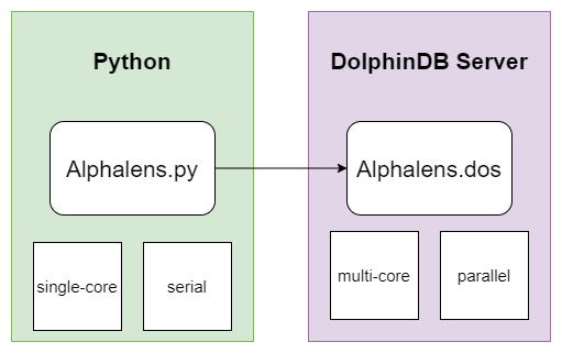
Alphalens is a factor analysis (evaluation) toolkit developed by Quantopian using Python. We implemented a module using DolphinDB’s scripting language (DLang), enabling users to run Alphalens directly on the DolphinDB Server. This not only improves convenience but also significantly enhances performance.

2. Alphalens Factor Analysis Module

2.1 Architecture and Basic Concepts

The usage of this module can be abstracted into three layers:

Data Storage Layer: Leverages DolphinDB’s distributed storage and computing engine to efficiently store and perform parallel computation on massive market and factor data.
Calculation and Analysis Layer: Implements Alphalens’ factor-analysis framework using DLang, handling complex logic such as data cleaning and portfolio evaluation.
Visualization and Interaction Layer: Uses Python’s Jupyter Notebook to present analysis results via interactive visualization tools.

For execution efficiency, when analyzing large numbers of single factors, DolphinDB’s built-in peach function can be used to concurrently invoke the analysis module. Combined with DolphinDB’s vectorized engines and distributed architecture, this ensures accuracy while delivering excellent performance.

For basic concepts, function names, parameters, and default values in DolphinDB’s Alphalens module are intentionally kept consistent with the Python version to minimize learning and migration costs.

For plotting, DolphinDB provides alphalens_plotting.py, which allows you to visualize results directly within Python. You can connect to DolphinDB Server via the Python API, call plot_create_full_tear_sheet or plot_create_returns_tear_sheet to obtain results, and finally use Pyfolio for rendering.

2.2 Typical Workflow

Calling the Alphalens module in DolphinDB typically involves three steps:

STEP 1: Prepare factor and market data.
STEP 2: Generate intermediate analysis results using get_clean_factor_and_forward_returns.
STEP 3: Call analysis functions to obtain output tables.

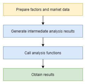
In the following sections, we will guide you through the entire process, from data preparation to intermediate result analysis, then to calling analysis functions, and finally realizing visualization through Jupyter notebook.

3. Data Preparation

Data quality is fundamental to quantitative investment. Understanding the data structure we use is the first step in starting the journey of factor research. In this chapter, we will introduce the stock trading data structure used in DolphinDB for this tutorial and construct the required factor features based on this raw data.

Note: Before starting, please download the file from the Appendix and place the alpahlens.dos file into <YOUR_DOLPHINDB_PATH>/server/modules/.

3.1 Generate Stock Data

We use genDayKDataAndSaveToDFS to generate simulated daily data for 5000 stocks, including fields such as symbol, trade date, open, high, low, close, volume, and VWAP. As the generation method is based on random simulation, limitations include:

Lack of realistic cross-asset correlations
Distribution differences from real markets
Inability to simulate holidays or unusual market conditions

It would be better to use your own real data, which you can import via the loadText function simply by modifying the field names accordingly.

This case uses a simple random number simulation method. It generates one year of simulated data and saves it to disk via the following script:

def genDayKDataAndSaveToDFS(securityIdNum, startDate, endDate) {
    securityId = lpad(string(1..securityIdNum), 6, "000000") $ SYMBOL
    tradeDate = table(getMarketCalendar("CFFEX", startDate , endDate) as tradeDate)
    // Use matrix and for loop way to generate simulated daily OHLC data.
    randStartOpen = double(int(randNormal(100, 30, size(securityId))))
    openList = [randStartOpen]
    for (day in tradeDate[1:]){
            openList.append!(openList[size(openList)-1] + randNormal(0, 2, size(securityId)))
    }
    res = cj(table(securityId as securityId), tradeDate)
    update res set open = flatten(openList.transpose())
    update res set high = round(open + rand(0.2, size(res)), 2)
    update res set low = round(high - rand(0.4, size(res)), 2)
    update res set close = round(open + norm(0, 0.1, size(res)), 2)
    update res set close = iif(close >= high, high, close)  // close should be less than high
    update res set close = iif(close <= low, low, close)  // close should be greater than low
    update res set volume = rand(100000, size(res))
    update res set amount = round(close*volume, 2)
    update res set vwap = round(close, 2)
    if (existsDatabase("dfs://alphalensTutorial")) {
        dropDatabase("dfs://alphalensTutorial")
    }
    db = database("dfs://alphalensTutorial", VALUE, `000001`000002)
    pt = db.createPartitionedTable(res, "dayK", `securityId)
    pt.append!(res)
}

// Generate simulated daily OHLC data
genDayKDataAndSaveToDFS(securityIdNum=5000, startDate=2024.01.01, endDate=2024.12.31)

// Observe daily OHLC data schema
select top 100 * from loadTable("dfs://alphalensTutorial", "dayK")

// securityId tradeDate	 open	high	low	    close	volume	amount	     vwap
// 000001	  2024.01.02 109	109.16	109.15	109.15	52,221	5,699,922.15 109.15
// 000001	  2024.01.03 107.41	107.44	107.08	107.43	65,895	7,079,099.85 107.43
// 000001	  2024.01.04 107.81	107.92	107.69	107.69	60,790	6,546,475.1	 107.69
// 000001	  2024.01.05 108.05	108.22	107.94	108.08	22,104	2,389,000.32 108.08
// 000001	  2024.01.08 106.83	106.84	106.59	106.76	78,025	8,329,949	 106.76

3.2 Data Preprocessing and Feature Extraction

Based on the raw data acquired, we need to further perform data cleaning and feature engineering to obtain factors that deeply possess investment reference value. Here we will use DolphinDB's built-in Ta-lib to compute four widely recognized technical analysis factors: RSI, CCI, PPO, and WILLR.

// Load Ta-lib technical indicator module
use ta
go

// Calculate factors
dayK = loadTable("dfs://alphalensTutorial", "dayK")
rsi = select tradeDate as tradetime, securityId as symbol, "rsi" as factorname, ta::rsi(close, timePeriod=14) as value from dayK context by securityId
cci = select tradeDate as tradetime, securityId as symbol, "cci" as factorname, ta::cci(high, low, close, timePeriod=14) as value from dayK context by securityId
ppo = select tradeDate as tradetime, securityId as symbol, "ppo" as factorname, ta::ppo(close, fastPeriod=12, slowPeriod=26) as value from dayK context by securityId
willr = select tradeDate as tradetime, securityId as symbol, "willr" as factorname, ta::willr(high, low, close, timePeriod=14) as value from dayK context by securityId

// Observe factor results
select top 100 * from rsi where value is not null

// tradetime	symbol	 factorname	   value
// 2024.01.22	000001	 rsi	       54.46
// 2024.01.23	000001	 rsi	       54.39
// 2024.01.24	000001	 rsi	       52.64
// 2024.01.25	000001	 rsi	       56.30
// 2024.01.26	000001	 rsi	       62.42

Technical analysis, as the most traditional method of quantitative analysis, aims to identify some regular fluctuation patterns from price trends, and based on this, make trend judgments and investment decisions. The four factors we use in this analysis and their general meanings are as follows:

RSI stands for Relative Strength Index, which measures market buying and selling power by analyzing the intensity of price changes and reversals.
CCI combines price, average price, and time to measure the extent of deviation of the current price from the past.
PPO is a Percentage Price Oscillator, analyzing the rise and fall of strength between long and short sides.
WILLR compares the current price with historical price ranges to discover overbought and oversold price ranges.

In practice, whether it's RSI, CCI, PPO, or WILLR, you often need to carefully adjust and optimize the parameters according to the underlying variety and investment strategy to fully leverage their effectiveness.

For more information about these factors, you may refer to:

RSI: Relative strength index
CCI: Commodity channel index
PPO: Percentage Price Oscillator (PPO): Definition and How It's Used
WILLR: Williams %R

For convenience of subsequent use, the factor data here is stored in a narrow-format table:

// Create factor database
def creatSingleModelDataBase(dbname, tbname) {
    if (existsDatabase(dbname)) {
        dropDatabase(dbname)
    }
    db = database(directory=dbname, partitionType=VALUE, partitionScheme=`factor1`factor2, engine="TSDB")
    factorPt = db.createPartitionedTable(table = table(1:0, ["tradetime", "symbol", "factorname", "value"], [TIMESTAMP, SYMBOL, SYMBOL, DOUBLE]), tableName=tbname, partitionColumns=["factorname"], sortColumns=[`tradetime])
    return factorPt
}

// Create factor database
factorPt = creatSingleModelDataBase("dfs://alphalensTutorialFactor", "factor")

// Write to factor database
factorPt.append!(rsi)
factorPt.append!(cci)
factorPt.append!(ppo)
factorPt.append!(willr)

4. Case Study: Single-Factor Analysis

As the most basic and critical link in multi-factor quantitative investment, the importance of single-factor analysis is self-evident. Only by thoroughly analyzing and evaluating a single factor can we fully recognize its actual predictive ability, sustainability, and other intrinsic characteristics, so as to prudently decide whether to include it in the investment portfolio and what weight should be assigned.

Alphalens provides a systematic and comprehensive single-factor analysis framework, capable of examining the performance of a factor from multiple dimensions, including returns, turnover rate, information ratio, and other perspectives allowing us to evaluate a factor's performance from multiple angles, thereby forming an accurate and comprehensive understanding and judgment of it.

We will take the classic technical factor RSI as an example, combined with Alphalens' powerful single-factor analysis capabilities, to demonstrate a complete workflow for conducting comprehensive factor analysis.

4.1 Prepare Data for Alphalens

The workflow of Alphalens single-factor analysis starts with the factor_data intermediate output produced by the get_clean_factor_and_forward_returns function. This function primarily requires two inputs: factor and prices. factor is a narrow-format table containing three columns ["date", "asset", "factor"]. prices is a wide-format table containing prices of all assets.

In DolphinDB, we can easily obtain these two inputs:

// Retrieve RSI factor data
factorPt = loadTable("dfs://alphalensTutorialFactor", "factor")
RSI = select tradetime as date, symbol as asset, value as factor from factorPt where factorname = "rsi"

// Observe RSI factor data
select top 100 * from RSI where factor is not null

// date		  	asset	factor
// 2024.01.22	000001	54.46
// 2024.01.22	000002	53.10
// 2024.01.22	000003	67.59
// 2024.01.22	000004	61.27
// 2024.01.22	000005	26.29

// Prepare closing price data
dayKPt = loadTable("dfs://alphalensTutorial", "dayK")
dayClose = select close from dayKPt pivot by tradeDate as date, securityId

// Observe daily OHLC data
select top 100 * from dayClose

// tradeDate   000001  000002	000003  000004	000005
// 2024.01.02  109.15  109.15	109.15  109.15	109.15
// 2024.01.03  107.43  107.43	107.43  107.43	107.43
// 2024.01.04  107.69  107.69	107.69  107.69	107.69
// 2024.01.05  108.08  108.08	108.08  108.08	108.08

4.2 Generate Intermediate Analysis Results

Once the input data is prepared, we can call the get_clean_factor_and_forward_returns function, which formats the data into a structure that Alphalens can use for subsequent analysis.

This function requires two key parameters: quantiles (quantiles) and holding periods (periods).

Alphalens evaluates factors by analyzing the correlation between factor values and their future returns. periods specifies the future return time range we aim to study. In this example, we focus on return performance across three holding periods: 1 day, 5 days, and 10 days. Alphalens will calculate the returns by holding each factor value within these three time periods respectively. However, note that when performing single-factor backtesting, Alphalens does not currently consider commission costs or price impact.

Financial market data often contains significant noise, making it difficult to directly identify the exact correlation between specific factor values and future returns. Therefore, Alphalens analysis relies on factor quantile statistics instead of raw factor values. Each day, factor values are divided into equal quantile buckets based on their distribution. This grouping improves the signal-to-noise ratio, clarifying the relationship between factors and returns.

The following code calls this function in DolphinDB to obtain intermediate analysis results:

// Load Alphalens module
use alphalens 
go

// Get intermediate analysis results
RSI_cleaned = select date(date) as date, asset, factor from RSI
cleanFactorAndForwardReturns = get_clean_factor_and_forward_returns(
    factor=RSI_cleaned,
    prices=dayClose,
    groupby=NULL,
    binning_by_group=false, 
    quantiles=5,  // Divide into 5 groups
    bins=NULL,  
    periods=[1, 5, 10],  // Holding periods
    filter_zscore=NULL,  // Outlier filtering
    groupby_labels=NULL,
    max_loss=0.35,
    zero_aware=false,
    cumulative_returns=true  // Cumulative returns
)

// Observe single factor analysis results
select top 100 date, asset, forward_returns_1D, forward_returns_5D, forward_returns_10D, factor, factor_quantile from cleanFactorAndForwardReturns

// For display convenience, only four decimal places are retained here
// date         asset   forward_returns_1D  forward_returns_5D  forward_returns_10D factor   factor_quantile
// 2024.01.22   000001  -0.0028             -0.0158             -0.0404             26.5229  1
// 2024.01.22   000002  -0.0045             -0.0754             -0.0734             27.2773  1
// 2024.01.22   000003  -0.0344             -0.0927             -0.0859             59.6302  4
// 2024.01.22   000005  0.0255              0.0378              0.056               67.2281  5

In the final output data, date and asset represent the date and asset information. The forward_returns_1D/5D/10D columns record future returns over the 1, 5, and 10-day holding periods, respectively. factor and factor_quantile denote the original factor values and their quantile groups.

This formatted result data prepares Alphalens for comprehensive analysis. For details on the parameters of get_clean_factor_and_forward_returns, see the official Alphalens documentation:

Alphalens—Alphalens 0.2.1+48.gad0be10 documentation

4.3 Obtain Single Factor Analysis Results

After generating the intermediate data for factor analysis, invoke Alphalens’ plot_create_full_tear_sheet function to conduct a comprehensive single-factor evaluation. This function outputs a dictionary containing multiple analysis results:

// Get factor analysis results
fullTearSheet = plot_create_full_tear_sheet(
    factor_data=cleanFactorAndForwardReturns, 
    long_short=true,  
    group_neutral=false,
    by_group=false  // Whether to analyze each group separately
)

Several key parameters are specified during the call:

long_short=true: Indicates calculating long/short portfolio.
group_neutral=false: Indicates not performing group neutralization.
by_group=false: Indicates analyzing all data as a whole, without group separation

The output dictionary fullTearSheet mainly contains three parts:

plot_turnover_tear_sheet focuses on trading-related metrics such as portfolio turnover.
plot_information_tear_sheet evaluates the predictive relationship between factors and returns, including key information-theoretic indicators such as the Information Coefficient (IC).
plot_returns_tear_sheet provides a comprehensive assessment of both absolute and relative portfolio performance across different holding periods.

// View the result table schema
for (key in fullTearSheet.keys()) {
    print(key)
    if (form(fullTearSheet[key]) == 5) {
        for (subKey in fullTearSheet[key].keys()) {
            print("    " + subKey)
        }
    }
}

// .
// ├── plot_turnover_tear_sheet
// │   ├── Mean_Factor_Rank_Autocorrelation
// │   ├── Mean_Turnover
// │   ├── autocorrelation
// │   └── quantile_turnover
// ├── plot_information_tear_sheet
// │   ├── mean_monthly_ic
// │   ├── ic_ts
// │   ├── Information_Analysis
// │   └── ic
// ├── plot_returns_tear_sheet
// │   ├── plot_cumulative_returns_1
// │   ├── cumulative_factor_data
// │   ├── cum_ret
// │   ├── std_spread_quant
// │   ├── returns_analysis
// │   ├── mean_ret_spread_quant
// │   ├── mean_quant_rateret_bydate
// │   ├── mean_quant_ret_bydate
// │   ├── factor_returns_
// │   └── mean_quant_rateret
// └── quantile_stats

Each part includes specific analysis items like means and quantiles, along with data for chart display. For example, quantile_stats offers common statistical indicators by group.

// View quantile_stats results
quantile_stats = fullTearSheet["quantile_stats"]
select top 100 * from quantile_stats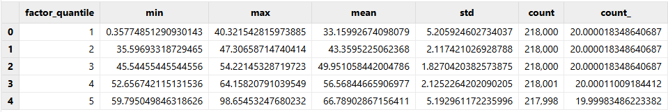

This comprehensive analysis allows us to evaluate a factor's actual performance from multiple perspectives.

Using the plot function, we start with a simple visualization of factor returns:

// View single factor long-short return curve
plot_cumulative_returns_1 = fullTearSheet["plot_returns_tear_sheet"]["plot_cumulative_returns_1"]
plot(plot_cumulative_returns_1.forward_returns_1D, plot_cumulative_returns_1.date)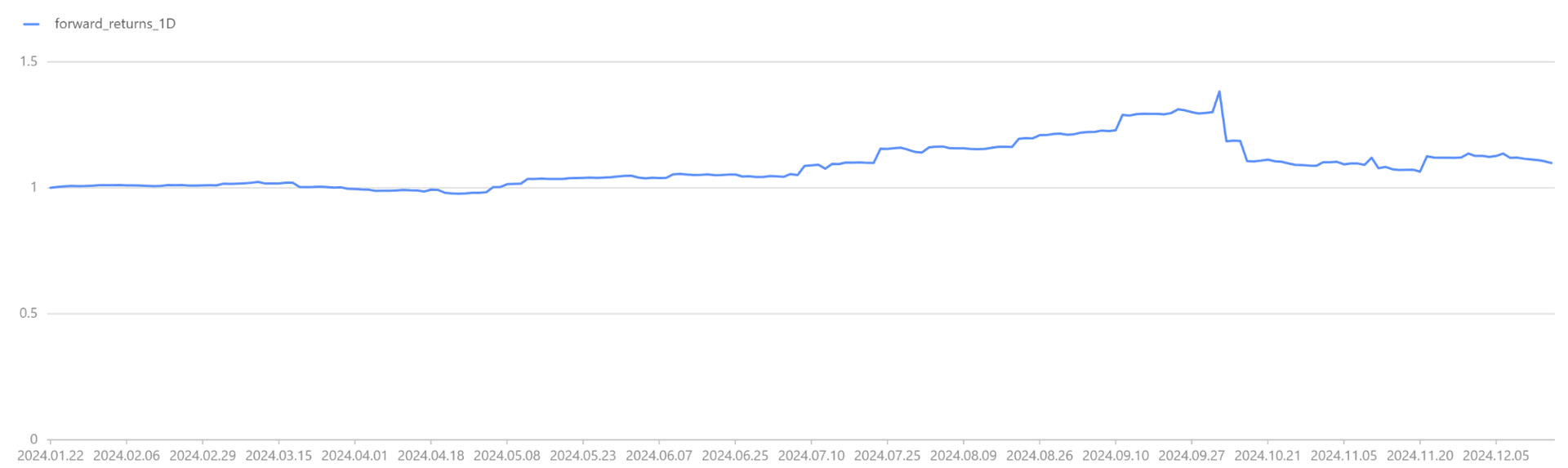

We share the result tables across sessions to support subsequent visualization tasks.

// Share factor result table for subsequent use
share(cleanFactorAndForwardReturns, `factor_data)

5. Visualization via Jupyter Notebook

Given the complexity and breadth of the single-factor analysis results, a powerful visualization tool is essential for presenting the information intuitively and enabling deeper insights. Jupyter Notebook serves as an ideal environment for this purpose.

This chapter demonstrates retrieving analysis results with the DolphinDB Python API and performing interactive visualization in Jupyter Notebook.

Note: Here we generate charts using the alphalens_plotting.py file. It is included in the Appendix, which enables you to reproduce the entire process.

5.1 Factor Distribution Analysis

This subsection uses the plot_quantile_statistics_table function to draw a statistical table of factors across quantile groups, showing their distribution. Observing this table reveals the range, mean, and median of factor values in each group, providing a foundation for further analysis.

First, load the required modules and establish a connection with DolphinDB using the following code:

import dolphindb as ddb
import pandas as pd
import matplotlib.pyplot as plt
import alphalens_plotting as plotting
import warnings

warnings.filterwarnings("ignore")

## Connect to DolphinDB server
s = ddb.session()
s.connect("localhost", 8848, "admin", "123456")

## Load Alphalens module in this session
s.run("use alphalens")

Use the plot_quantile_statistics_table function to draw the table and observe the factor distribution across groups:

## Factor Distribution Analysis
script_plot_quantile_statistics_table = '''
    plot_quantile_statistics_table(factor_data)
'''
ret = s.run(script_plot_quantile_statistics_table)
plotting.plot_quantile_statistics_table(ret)

5.2 Factor Returns Analysis

Return analysis is the core component of the single-factor evaluation workflow. In this subsection, we use the plot_create_returns_tear_sheet function to generate a suite of factor-return visualizations, including cumulative return curves for various holding periods and return distributions by quantile groups. These visual outputs enable intuitive assessment of the factor’s profitability and behavior under different market conditions. Such insights guide refinement of investment strategies, such as selecting optimal holding periods or adjusting factor use across market environments.

## Factor Returns Analysis
script_plot_create_returns_tear_sheet = '''
    plot_create_returns_tear_sheet(factor_data,by_group=false, long_short=true, group_neutral=false)
'''
ret = s.run(script_plot_create_returns_tear_sheet)
plotting.create_returns_tear_sheet(ret, save_name="returns_tear_sheet.png", save_dpi=500)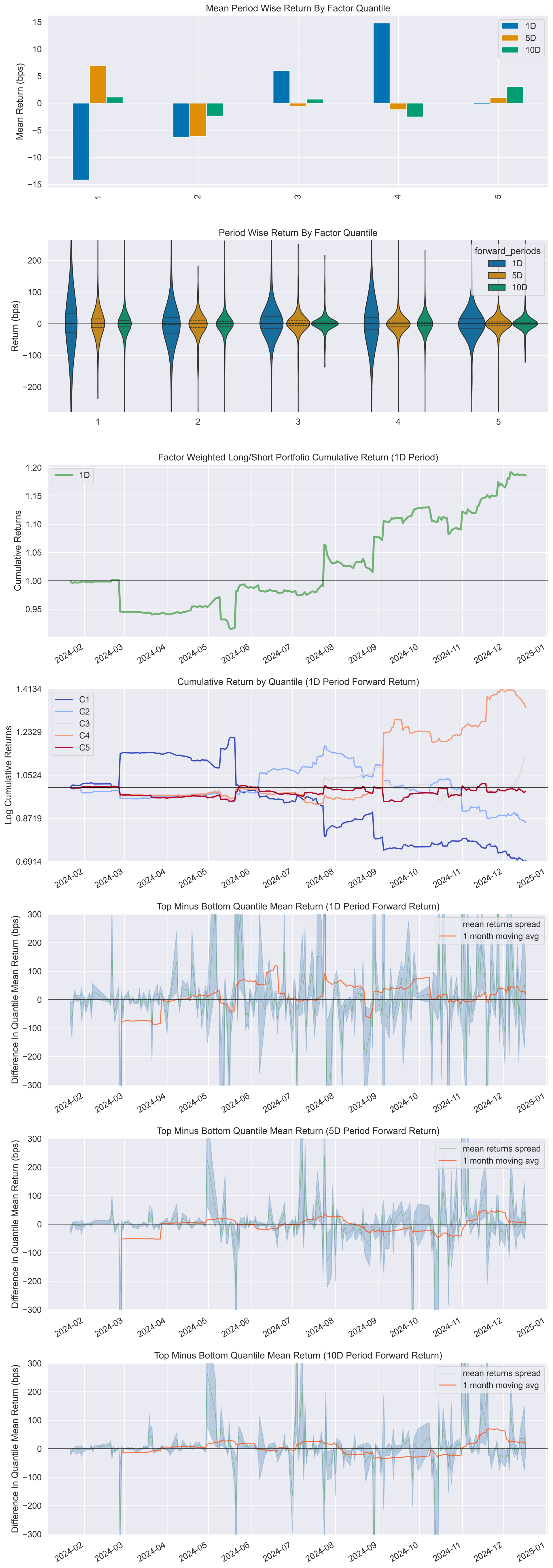

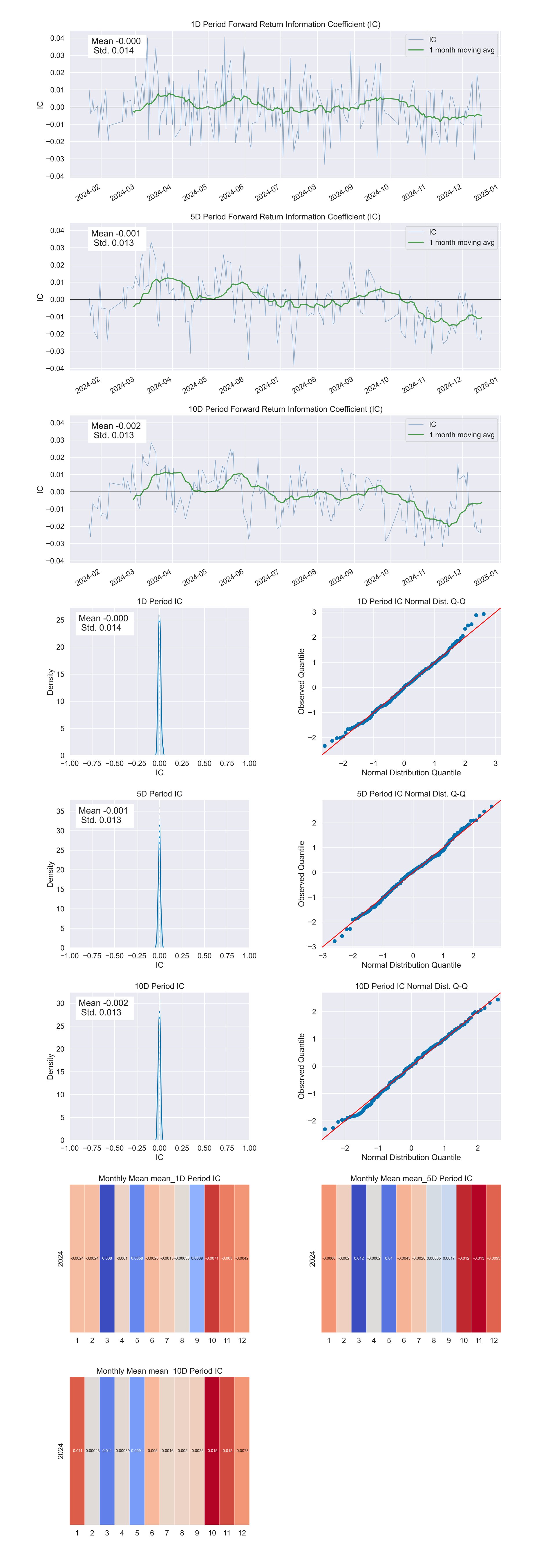
5.3 Factor IC Analysis

IC (Information Coefficient) measures factor predictive power by reflecting the correlation between factor values and actual returns. An effective factor has a high IC value and maintains stability over time. We use the create_information_tear_sheet function to generate charts for IC analysis, including IC time series and monthly IC mean.

Analyzing the above IC charts allows us to evaluate this factor's predictive power and effectiveness comprehensively and determine its reliability and investment value. For example, a factor that maintains a high, stable IC over time likely warrants attention.

## Factor IC Analysis
script_plot_create_information_tear_sheet = '''
    create_information_tear_sheet(factor_data, group_neutral=false, by_group=false)
'''
information_tear_sheet = s.run(script_plot_create_information_tear_sheet)
plotting.create_information_tear_sheet(information_tear_sheet, save_name="information_tear_sheet.png", save_dpi=500)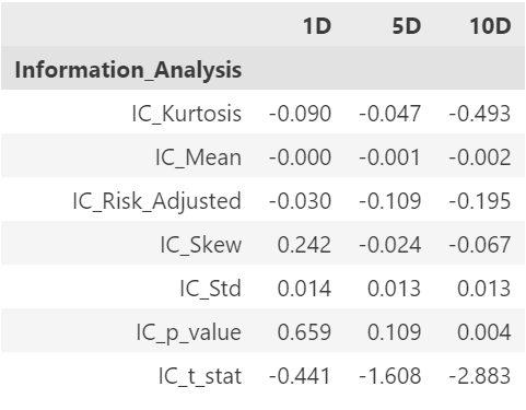

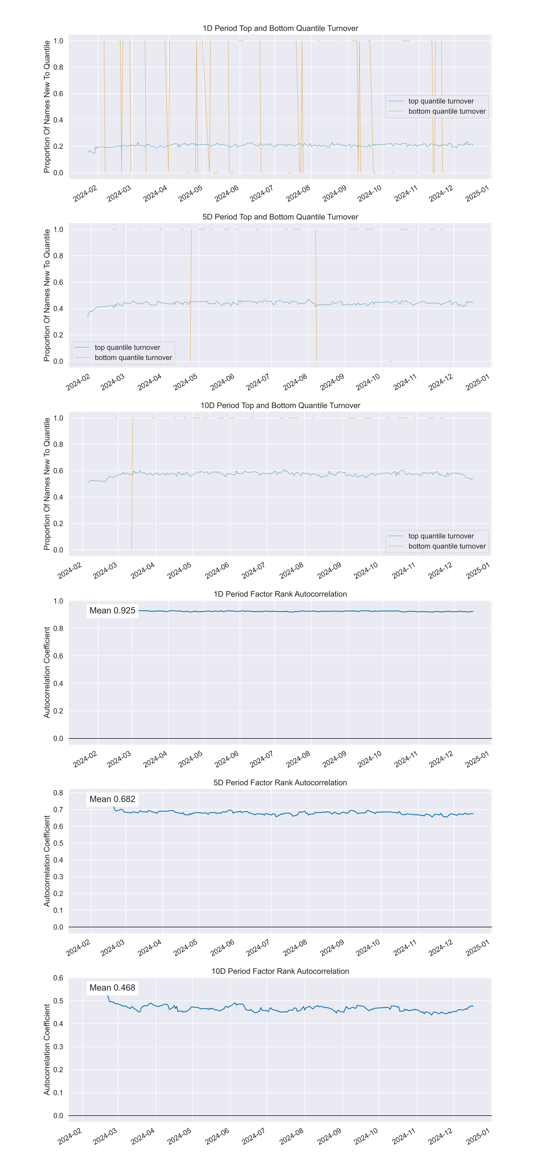
5.4 Factor Turnover Analysis

Portfolio turnover is a key indicator for evaluating trading activity and execution costs. High turnover indicates frequent trading, increasing costs and potential drawbacks. Low turnover may prevent timely portfolio adjustments, missing profit opportunities. This subsection uses the create_turnover_tear_sheet function to generate visualization charts showing average portfolio turnover and quantile turnover across holding periods, aiding evaluation of trading activity and execution costs.

## Factor Turnover Analysis
script_plot_create_turnover_tear_sheet = '''
    create_turnover_tear_sheet(factor_data, turnover_periods_=NULL)
'''
turnover_tear_sheet = s.run(script_plot_create_turnover_tear_sheet)
plotting.create_turnover_tear_sheet(turnover_tear_sheet, save_name="turnover_tear_sheet.png", save_dpi=500)


factor_quantile	1	5	10
Quantile_5_Mean_Turnover	0.2068110599078341	0.4387934272300466	0.5752259615384608
Quantile_4_Mean_Turnover	0.4671612903225802	0.6975492957746474	0.7520432692307693
Quantile_3_Mean_Turnover	0.5238525345622125	0.7296760563380287	0.7740288461538462
Quantile_2_Mean_Turnover	0.4672466519655457	0.6974380220718241	0.7533617680396527
Quantile_1_Mean_Turnover	0.2066286424673523	0.43826235155343113	0.5721353565103563


periods	Mean_Factor_Rank_Autocorrelation
1	0.9245
5	0.6802
10	0.4666

6. Summary and Outlook

6.1 Advantages of Alphalens + DolphinDB

This case demonstrated how to use the Alphalens module in DolphinDB for single-factor analysis and highlighted the significant benefits of integrating Alphalens, a professional single-factor analysis framework, with DolphinDB, a high-performance engine for time-series data:

Improved data processing efficiency: DolphinDB, a distributed database optimized for financial time-series data, efficiently stores and processes massive financial datasets, providing a foundation for subsequent analysis.
Comprehensive analysis functions: Alphalens, a professional quantitative analysis library, covers core dimensions including factor distribution, return analysis, IC analysis, and turnover evaluation, ensuring comprehensive analysis results.
Intuitive visualization exploration: Visualization based on Python and Jupyter notebook renders analysis results more interactive and interpretable, aiding factor performance optimization.
Seamless tool chain integration: DolphinDB's Alphalens module combines DolphinDB's data processing capabilities with Alphalens' quantitative analysis functions, forming an efficient tool chain for single-factor investment research.

6.2 Future Trends of Quantitative Investment

Single-factor analysis is a cornerstone of quantitative investment but represents only part of the field. As technology advances, quantitative investment evolves toward diversification and intelligence:

The rise of high-frequency trading:
- Real-time market signal acquisition enables capturing fleeting trading opportunities. DolphinDB's built-in stream computing engine plays a key role in this process. DolphinDB Stream Computing Introduction
Increasing importance of portfolio optimization:
- Optimizing portfolios to maximize returns while controlling risks is becoming a core demand for investors. DolphinDB's optimization solver functions provide strong support for this. Portfolio Optimization: A Guide to DolphinDB Optimization Solvers
Automated factor mining as a research focus:
- DolphinDB launched the Shark GPLearn high-performance factor mining platform. Unlike traditional manual factor design and feature engineering, Shark reads data directly from the database, uses genetic algorithms for automatic factor mining, and employs GPU acceleration for fitness calculations, improving mining efficiency.

The future of quantitative investment will feature intelligent decision-making, multi-strategy integration, and cross-domain collaboration. DolphinDB will continue to innovate in line with these trends, and deliver valuable products and services to investors.

Appendix

dolphindbAlpahlensTutorial.zip