Shark for Monte Carlo Simulation-based Pricing
As Moore’s Law approaches its physical limits, improvements in single-core CPU performance have slowed down, while the rapid growth of big data and artificial intelligence has led to an exponential increase in computational demand. To address this challenge, leveraging heterogeneous processors such as GPUs and FPGAs for acceleration has become a major technical trend. This tutorial introduces Shark, DolphinDB’s CPU–GPU heterogeneous computing platform, and demonstrates how it accelerates script execution in FICC (Fixed Income, Currencies and Commodities) applications such as snowball option pricing and coupon rate determination.
1. Introduction to Shark
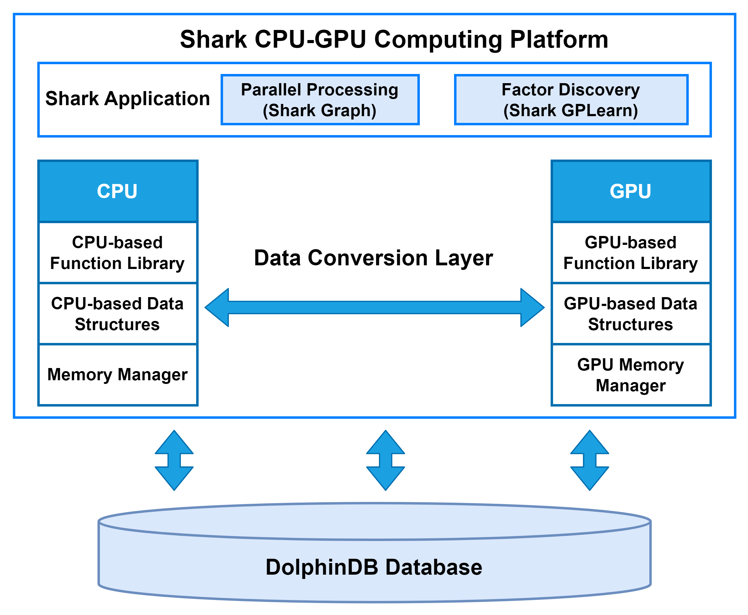
Shark is a CPU–GPU heterogeneous computing platform introduced in DolphinDB 3.0. Built on DolphinDB’s high-performance storage system, Shark deeply integrates GPU parallel computing power to deliver significant acceleration for compute-intensive workloads. Based on a heterogeneous computing framework, Shark consists of two core components:
-
Shark Graph: Accelerates the execution of DolphinDB scripts with GPU parallelism, enabling efficient parallel processing of complex analytical tasks.
-
Shark GPLearn: Designed for quantitative factor discovery, it supports automated factor discovery and optimization based on genetic algorithms.
By leveraging these capabilities, Shark effectively overcomes the performance limitations of traditional CPU computation and greatly enhances DolphinDB’s efficiency in large-scale data analytics, such as high-frequency trading and real-time risk management.
1.1 Architecture of the Shark Computing Platform
The data conversion layer in Shark is responsible for managing data transfer between host memory and device memory.
At the start of computation, the CPU reads data from disk into host memory and transfers it to device memory for processing. Once GPU computation is completed, the results are copied back to host memory and then written to the DolphinDB database via the CPU.
On the GPU side, Shark implements fundamental data forms such as vectors, matrices, and tables. Based on these, the Shark GPU function library supports a wide range of DolphinDB functions, enabling complex operations to run on the GPU directly from DolphinDB scripts. To further optimize performance, Shark incorporates a custom device memory manager that efficiently handles memory allocation and recycling during computation.
1.2 Data Transfer Module
The data transfer module serves as the core bridge for CPU–GPU communication in Shark, handling all data interactions and transfers for higher-level applications. In complex data analytics tasks, the efficiency of data transfer between device memory and host memory often becomes the performance bottleneck.
Taking GPU-to-host memory data copy as an example, the transfer occurs in two stages:
- Data is copied from pageable memory to pinned memory, with transfer speed limited by host memory bandwidth.
- Data is then transferred from pinned memory to device memory via the PCIe bus, with speed constrained by PCIe bandwidth.
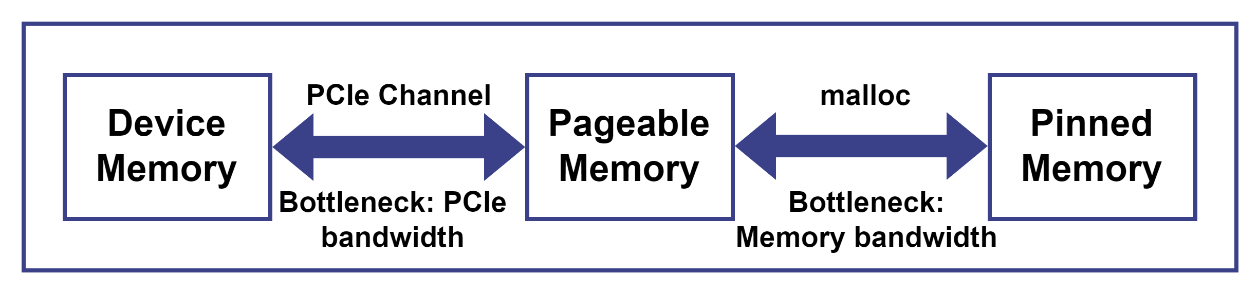
The combined latency of these two stages constitutes the overall communication overhead. In real-time high-frequency factor computations, the per-transfer data is small and GPU parallel computation time is extremely short; measurements show that nearly 90% of the total time is spent on host-device data transfers. When the GPU can process millions of tasks per second, this idle time due to communication latency represents a significant hidden cost.
Since the copy process is multi-staged, with each stage needing to complete before the next begins, Shark applies a classic computer optimization technique—pipelining—to improve data transfer efficiency and reduce the impact of communication latency on overall computational performance.
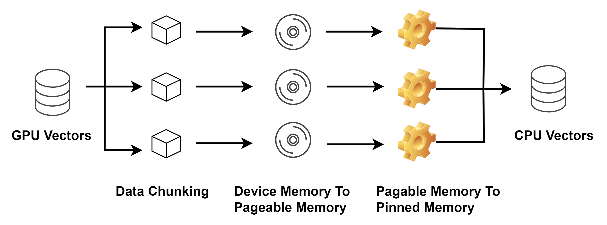
Shark first divides the data into 2MB blocks and employs multi-threaded block-wise copying, with each thread handling multiple blocks. Within a single thread, data is first copied from device memory to pageable memory, and then from pageable memory to pinned memory. By adopting this pipelined processing approach, Shark significantly improves the utilization of host memory bandwidth, while incurring only a modest PCIe bandwidth overhead.
2. Shark Graph
The application examples in this tutorial primarily leverage Shark Graph for GPU-accelerated computation. For details on Shark GPLearn and automated factor discovery, refer to the relevant tutorials.
2.1 Function Overview
Numerous computationally intensive tasks, such as factor calculation in quantitative trading, snowball option pricing and coupon rate determination in FICC, and high-dimensional Monte Carlo simulations, are well-suited for GPU acceleration. To meet this requirement, Shark provides Shark Graph.
Many existing DolphinDB scripts can be executed on the GPU without modification.
By simply adding the @gpu annotation before the functions,
Shark automatically schedules and executes the script on the GPU, achieving
acceleration. This approach allows researchers to utilize GPU computing without
writing CUDA code and facilitates seamless migration of existing DolphinDB
scripts to GPU execution.
Shark Graph supports the following data types and forms:
- Data types: BOOL, CHAR, SHORT, INT, LONG, FLOAT, DOUBLE
- Data forms: scalar, vector, matrix, table. Note that indexed matrices are not yet supported, and only in-memory tables are supported.
Shark Graph supports a subset of Dlang syntax for GPU execution, including
for loops, if-else statements,
break, continue, assignment, and multiple
assignments. SQL statements cannot run directly on the GPU and must be wrapped
in a user-defined function for execution.
Key advantages
- Low learning curve: Simply adding the annotation enables GPU acceleration using DolphinDB scripts.
- Low migration cost: Most DolphinDB scripts and data forms can run on the GPU with minimal adjustments.
- High computational efficiency: For computationally intensive financial tasks, such as Monte Carlo-based snowball option pricing, Shark Graph can achieve up to 200× speedup compared with Python.
2.2 Workflow
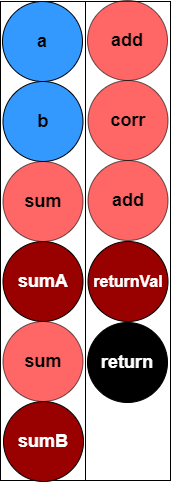
For user-defined function scripts, Shark Graph first parses the script and converts it into a directed acyclic graph (DAG), as illustrated below:
@gpu
def factor(a, b){
  sumA = sum(a)
  sumB = sum(b)
  return sumA + sumB + corr(a, b)
}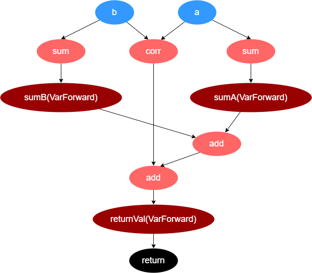
Shark Graph performs a breadth-first traversal of the DAG and places the nodes into a work queue. Nodes are executed sequentially by dequeuing them from the work queue.
When Shark Graph executes a node that represents an operator, it first determines whether the operator should run on the CPU or GPU. The operator's dependent parameters are then copied to the appropriate memory (CPU or GPU) by the data transfer module. Once the parameters are available, the operator executes, leveraging GPU acceleration if assigned to the GPU.
Once all nodes in the work queue have been processed, the execution of the user-defined function is complete. Shark Graph then copies the return values from device memory back to host memory and returns them to the caller.
2.3 VWAP Calculation
For quick deployment of the test environment, refer to Quick Start Guide for Shark GPLearn.
The following example demonstrates how to compute the VWAP indicator using Shark Graph:
- Generate simulated market data as a matrix (price and
volume).
def simulation(days, nSymbols){ """ Generate simulated price and volume data """ // Generate simulated trading time: assume 9:30–11:30 in the morning and 13:00–15:00 in the afternoon timeList = (09:30:00 + 3*0..2400) <- (13:00:00 + 3*0..2400) timeList = each(concatDateTime{, timeList}, days).flatten() // Get the total number of time points (timestamps) in the simulated trading period nTimes = size(timeList) // Simulate the price matrix // Assign a random initial price to each symbol initPrice = rand(100.0, nSymbols) initPriceMatrix = flip(take(initPrice, nSymbols*nTimes)$nSymbols:nTimes) // Generate a random return series for each symbol returnMatrix = norm(0, 0.01, nTimes:nSymbols) // Calculate the simulated price matrix priceMatrix = initPriceMatrix * cumprod(1 + returnMatrix) priceMatrix.rename!(string(timeList), "c"+lpad(string(1..nSymbols), 6, "0")) priceMatrix = round(priceMatrix, 3) // Simulate the volume matrix volumeMatrix = 100*rand(100, nSymbols*nTimes)$nTimes:nSymbols volumeMatrix.rename!(string(timeList), "c"+lpad(string(1..nSymbols), 6, "0")) return priceMatrix, volumeMatrix } // Simulated date days = 2025.01.01 // Number of simulated symbols nSymbols = 6000 // Generate simulated data price, volume = simulation(days, nSymbols) - Write VWAP calculation scripts for both CPU and GPU execution. If the
function only involves data types and aggregate functions supported by Shark
Graph, add the
@gpuannotation to enable GPU acceleration.def vwap_cpu(price, volume, window){ result = msum(price * volume, window) / msum(volume, window) return result } @gpu def vwap_gpu(price, volume, window){ result = msum(price * volume, window) / msum(volume, window) return result } - Run the scripts and compare their
performance.
// Execution time on CPU
timer{
    result = vwap_cpu(price, volume, 20)
}
// Execution time on GPU
timer{
    result = vwap_gpu(price, volume, 20)
}
The results show that Shark Graph provides substantial speed improvements compared with the CPU implementation.
// Execution time on CPU
Time elapsed: 444.387 ms
// Execution time on GPU
Time elapsed: 40.881 ms
3. Application
3.1 Typical Snowball Option Example
Snowballs are autocallable structured products with an early redemption feature. The contract is redeemed when the underlying asset price reaches a specified barrier on predetermined observation dates. Due to typically higher coupon rates, snowball products have gained significant investor interest in recent years, with the market continuously expanding.
Snowball options, as a key component of snowball products, involve the investor selling a put option with complex barrier conditions: limited gains when the underlying asset rises, and potential losses reflecting the asset decline.
To facilitate understanding, a classic snowball option contract is used to illustrate the payoff differences compared with a standard long position or index fund. The table below summarizes a typical contract structure and key parameters.
| Product Element | Description |
|---|---|
| Underlying asset | CSI 500 Index (000905.SH) |
| Observation period | 1 year; monthly knock-out observation at month-end and daily knock-in observation, starting from the third month |
| Option structure | Automatic early redemption with knock-in and knock-out conditions |
| Notional principal | 1,000,000 |
| Knock-out level | Initial price × 103% |
| Knock-in level | Initial price × 80% |
| Knock-out coupon | 25% (annualized) |
| Dividend coupon | 25% (annualized) |
| Knock-out event | On any knock-out observation date, the underlying closes ≥ knock-out level |
| Knock-in event | On any knock-in observation date, the underlying closes < knock-in level |
| Payoff calculation |
|
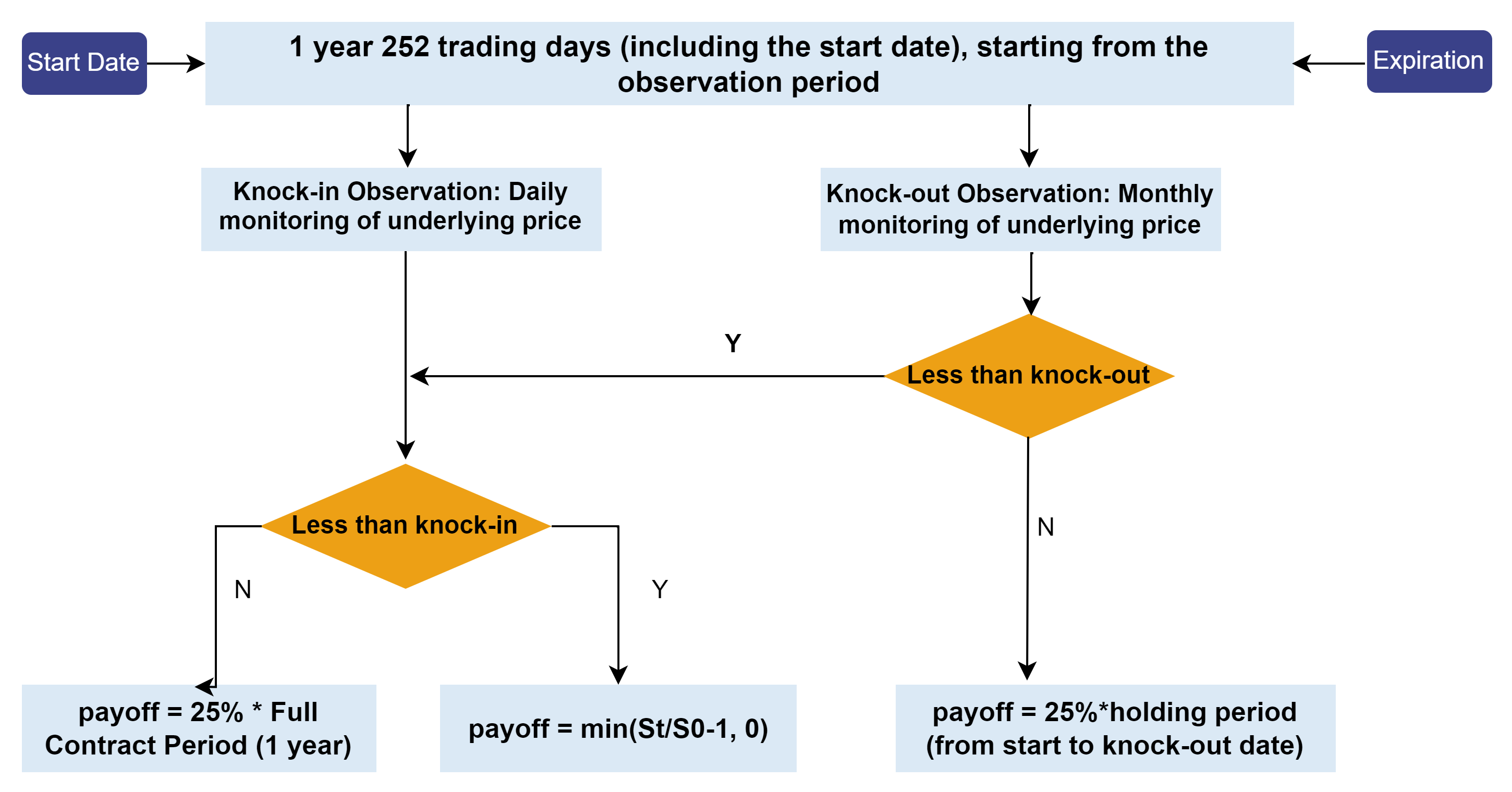
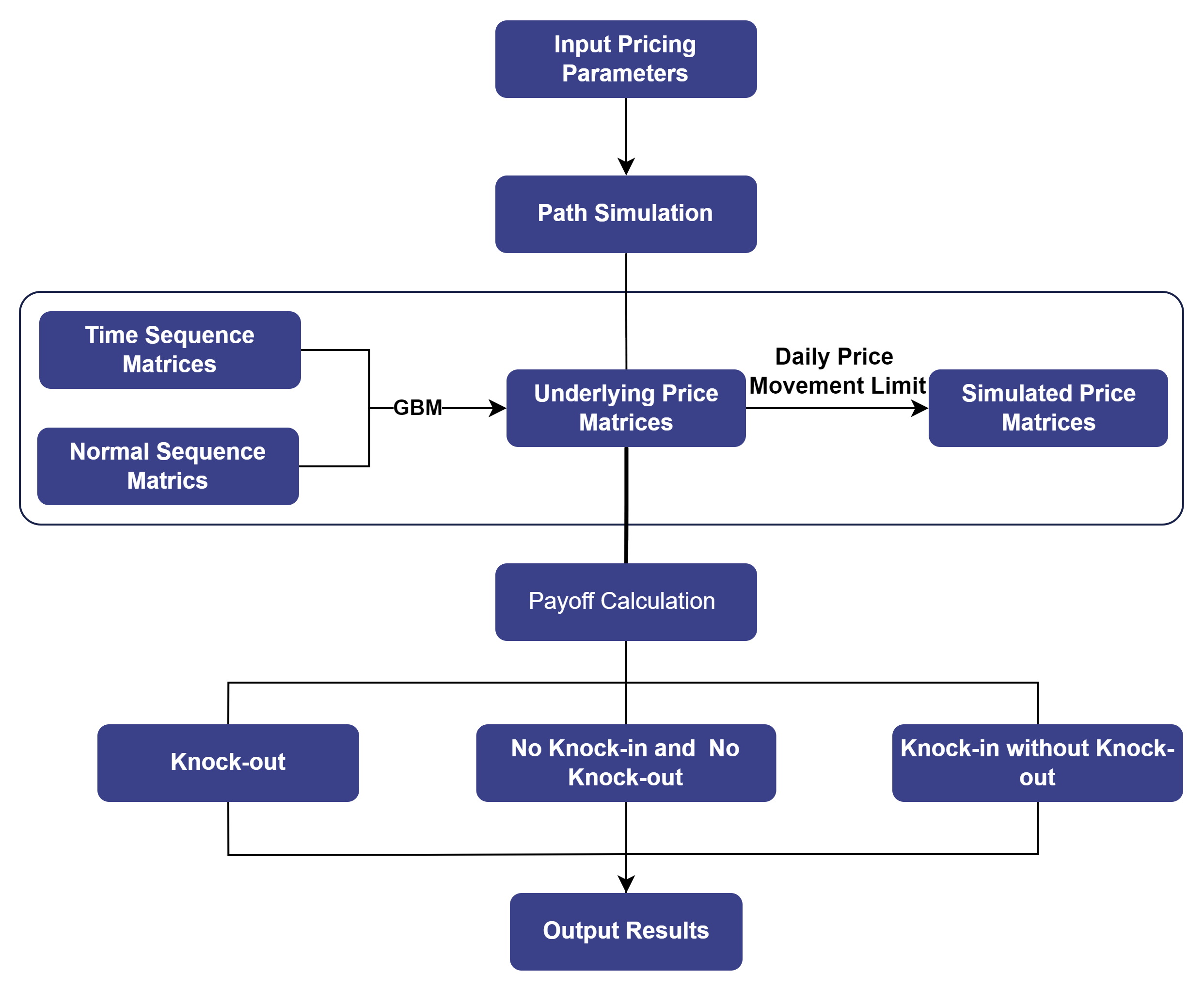
For a typical snowball option contract, the buyer’s final payoff can be classified into three scenarios:
- Early redemption: If the CSI Index closes at ≥ 103% of the initial price on any monthly observation date, the knock-out condition is triggered. The contract settles with the knock-out coupon, yielding principal + 25% coupon.
- No knock-in, no knock-out: If the CSI Index closes below 103% of the initial price on all monthly knock-out observation dates, and remains ≥ 80% of the initial price on all daily knock-in observation dates, neither knock-in nor knock-out is triggered. The contract settles with the dividend coupon, yielding principal + 25% coupon.
- Knock-in without knock-out: If the CSI Index closes below 80% of the initial
price on any daily knock-in observation date, and below 103% on all monthly
knock-out observation dates, only the knock-in condition is triggered. The
contract payoff at maturity is
min((final price / initial price −
                            1), 0) × notional
. Denoting the final price as St and the initial price as S0, the payoff is−max(S0−St,0), equivalent to selling a put option with strike S0.
These scenarios are summarized in the payoff flowchart below:
For the issuer, payoffs are the inverse of the buyer’s. The issuer’s goal is to determine an appropriate coupon rate for the snowball product given a target return and other contract parameters.
3.2 Option Pricing Models
The commonly used numerical methods for option pricing include the Black-Scholes (BS) model, the finite difference method, and the Monte Carlo simulation.
- The BS model is a classical analytical approach. It constructs a risk-free hedging portfolio, derives the partial differential equation (PDE) satisfied by the option price, and solves it for a closed-form solution. The finite difference method discretizes the PDE into finite differences and solves the resulting tridiagonal system on a grid. Although accurate, it involves relatively complex computations.
- The Monte Carlo method assumes that the underlying asset price follows a stochastic process, typically Geometric Brownian Motion (GBM), and estimates the option value by simulating a large number of price paths. It is easy to implement and particularly suitable for high-dimensional, path-dependent, and multi-asset options, since its error convergence rate is independent of the problem’s dimensionality.
The snowball option is a type of exotic option, typically priced using Monte Carlo simulations. The basic principle is as follows:
Under the risk-neutral measure, the underlying asset price follows a GBM:
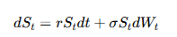
where St is the asset price at time t, r is the risk-free interest rate, σ is the volatility, and Wt is a Wiener process. In discrete form, the price paths of the underlying asset can be generated using the following recursive formula:
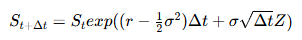
Once the simulated price paths are obtained, the snowball option buyer calculates the present value of each path according to its payoff structure. The option’s theoretical value is then the average of these discounted payoffs.
For the issuer, the objective is to determine the coupon rate (including both the knock-out and dividend coupons) that achieves a target yield. The same Monte Carlo framework is used to simulate price paths and compute the option value, while the coupon rate is iteratively adjusted—typically using the bisection method—until the desired yield is met.
3.3 Scenario 1: Snowball Option Pricing
Based on the Monte Carlo simulation method introduced above, the snowball option pricing process can be summarized as follows.
3.3.1 Path Simulation
The seq and repmat functions are used to
construct time sequence matrices with a specified number of paths. A
normally distributed random matrix is generated using the
norm function. Both matrices are then substituted into
the Black-Scholes model to generate simulated underlying price paths.
To better reflect real market conditions, this example imposes a ±10% daily price movement limit. The sample code is shown below.
@gpu
def simulation(S, r, T, sigma, N, days_in_year){
// Calculate the daily time interval (in years)
dt = 1 \ days_in_year
// Convert maturity time to days
Tdays = T*days_in_year
// Number of trading days per month (used for monthly knock-out observation)
monthDay = int(days_in_year/12)
all_t = dt*(0..Tdays)
// Each column represents a time series, with N columns in total
dtMatrix = repmat(matrix(all_t),1,N)
normMatrix = norm(0,1,(Tdays+1)*N)$(Tdays+1):N
normMatrix = normMatrix * (all_t>0)
// Each column represents one simulated price path, with N columns in total
ST = S * exp((r-0.5*sigma*sigma)*dtMatrix + sigma*sqrt(dt)*cumsum(normMatrix))
Spath = ST[1..Tdays, ]
// Apply daily price limits (10% up/down)
prevPrice = ST[0..(Tdays-1), ]
uplimit = prevPrice*1.1
lowlimit = prevPrice*0.9
Spath = iif(Spath > uplimit, uplimit, iif(Spath < lowlimit, lowlimit, Spath))
return Spath
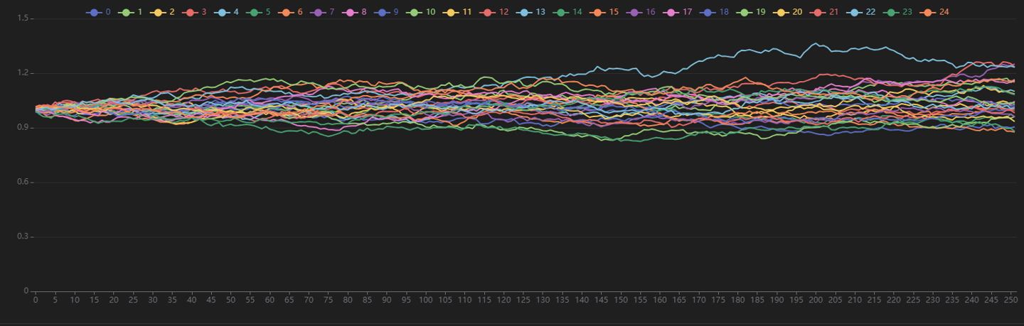
}The following figure visualizes the simulated price path matrix Spath, showing only the first 25 paths.
3.3.2 Pricing Function
As described earlier, a user-defined function that uses only Shark
Graph–supported data forms and functions can be executed on the GPU by
simply adding the @gpu annotation.
Once the underlying price matrix is obtained, DolphinDB’s vectorized operations allow efficient evaluation of each price path’s payoff according to the snowball option’s payoff structure. The average of all simulated payoffs represents the estimated option price.
The following shows the main function for snowball option pricing in Shark Graph.
@gpu
def snowball_pricing(S,r,T,sigma,N,coupon,k_out,k_in,lock_period,days_in_year){
    // Convert maturity time to days
    Tdays = T*days_in_year
    // Number of trading days per month (used for monthly knock-out observation)
    monthDay = int(days_in_year/12)
    Spath = simulation(S, r, T, sigma, N, days_in_year)
    // Construct the time indices for knock-out observation (after lock-up period)
    observation_out_idx = monthDay*(1..(Tdays/monthDay))
    observation_out_idx = observation_out_idx[observation_out_idx>lock_period]-1
    // Determine if knock-out occurs each month
    knockOutMatrix = Spath[observation_out_idx, ]>=k_out
    // Get the knock-out dates
    knock_out_day = observation_out_idx*knockOutMatrix
    // Find the first knock-out date
    knock_out_day = min(knock_out_day[knock_out_day>0])
    // Determine if knock-in occurs
    knock_in_day = sum(Spath < k_in)

    // Calculate payoff:
    // Scenario 1: Upward knock-out occurs: the snowball product terminates early according to the contract
    // Investor payoff = annualized coupon * holding period (in years)
    payoff1 = coupon*knock_out_day/days_in_year*exp(-r * knock_out_day/days_in_year)
    // Scenario 2: Neither knock-out nor knock-in occurs: product matures normally
    // Investor payoff = annualized coupon * holding period
    payoff2 = coupon * exp(-r * T)
    // Scenario 3: Only downward knock-in occurs, no upward knock-out, and underlying price at maturity is below initial price
    // Product matures normally; the knock-in put option is in-the-money, investor bears loss due to asset decline
    payoff3 = (last(Spath) - S)*exp(-r * T)
    // Determine the payoff for each price path
    payoff = iif(knock_out_day>0, payoff1,
             iif(knock_in_day==0, payoff2,
             iif(last(Spath)<S, payoff3, 0)))

    // Count knock-out occurrences
    knock_out_times = sum(knock_out_day>0)
    // Count occurrences of neither knock-out nor knock-in
    existence_times = sum(knock_out_day<=0&&knock_in_day==0)
    // Count knock-in occurrences
    knock_in_times = sum(knock_out_day<=0&&knock_in_day>0)
    // Count loss occurrences
    lose_times = sum(knock_out_day<=0&&knock_in_day>0&&last(Spath)<S)
    return payoff, knock_out_times, knock_in_times, existence_times,lose_times
}
The function returns:
- payoff: a vector of option values for each simulated path
- knock_in_times: number of knock-in events triggered
- knock_out_times: number of knock-out events triggered
- existence_times: number of paths that reached maturity without barrier events
- lose_times: number of loss occurrences
3.3.3 Function Parameters
Key parameters in the Monte Carlo simulation include the number of simulated paths, initial underlying price, knock-in and knock-out levels, and volatility. These parameters can be configured through function inputs. The parameter definitions used in this example are summarized in the table below:
| Parameter & Variable | Description |
|---|---|
| Number of simulated paths (N) | Number of asset price paths generated by the Monte Carlo simulation |
| Initial price (S) | Initial price of the underlying asset for the snowball option |
| Trading days per year (days_in_year) | Total number of trading days in a year |
| Lock-up period (lock_period) | Lock-up period in days as specified in the snowball option contract |
| Knock-in barrier (k_in) | Knock-in barrier price specified in the snowball option contract |
| Knock-out barrier (k_out) | Knock-out barrier price specified in the snowball option contract |
| Risk-free rate (r) | User-specified risk-free interest rate |
| Time to maturity (T) | Maturity of the snowball option, in years |
| Volatility (sigma) | Annualized volatility of the underlying asset |
| Coupon rate (coupon) | Annualized coupon rate of the snowball option (assuming knock-out coupon = dividend coupon) |
The parameter configuration and sample execution code are provided as follows:
N = 300000          // Number of simulation paths
S = 1.0             // Initial price of the underlying asset
k_in = 0.85         // Knock-in barrier
k_out = 1.03        // Knock-out barrier
T = 1               // Time to maturity (years)
days_in_year = 252  // Number of trading days per year
sigma = 0.13        // Annualized volatility of the underlying asset
r = 0.03            // Risk-free interest rate (annualized)
coupon = 0.2        // Coupon rate (annualized)
lock_period = 90     // Lock-up period (days)

timer payoff, knock_out_times, knock_in_times, existence_times, lose_times = snowball_pricing(S, r, T, sigma, N, coupon, k_out, k_in, lock_period, days_in_year)
print("Snowball value:", avg(payoff))
print("Knock-out probability:", knock_out_times \ N)
print("Probability of neither knock-in nor knock-out:", existence_times \ N)
print("Probability of knock-in without knock-out:", knock_in_times \ N)
print("Loss probability:", lose_times \ N)
3.3.4 Pricing Results
The output of GPU-accelerated pricing with Shark Graph is shown below. Under the given parameters, the snowball option achieves an expected annualized yield of 5% with a 73% probability of knock-out, indicating favorable investment potential. The total computation time for pricing is less than 40 ms.
Time elapsed: 36.827 ms

Snowball value: 0.050549256728865

Knock-out probability: 0.737543333333333

Probability of neither knock-in nor knock-out: 0.136706666666667

Probability of knock-in without knock-out: 0.12575

Loss probability: 0.123776666666667
3.4 Scenario 2: Snowball Option Design
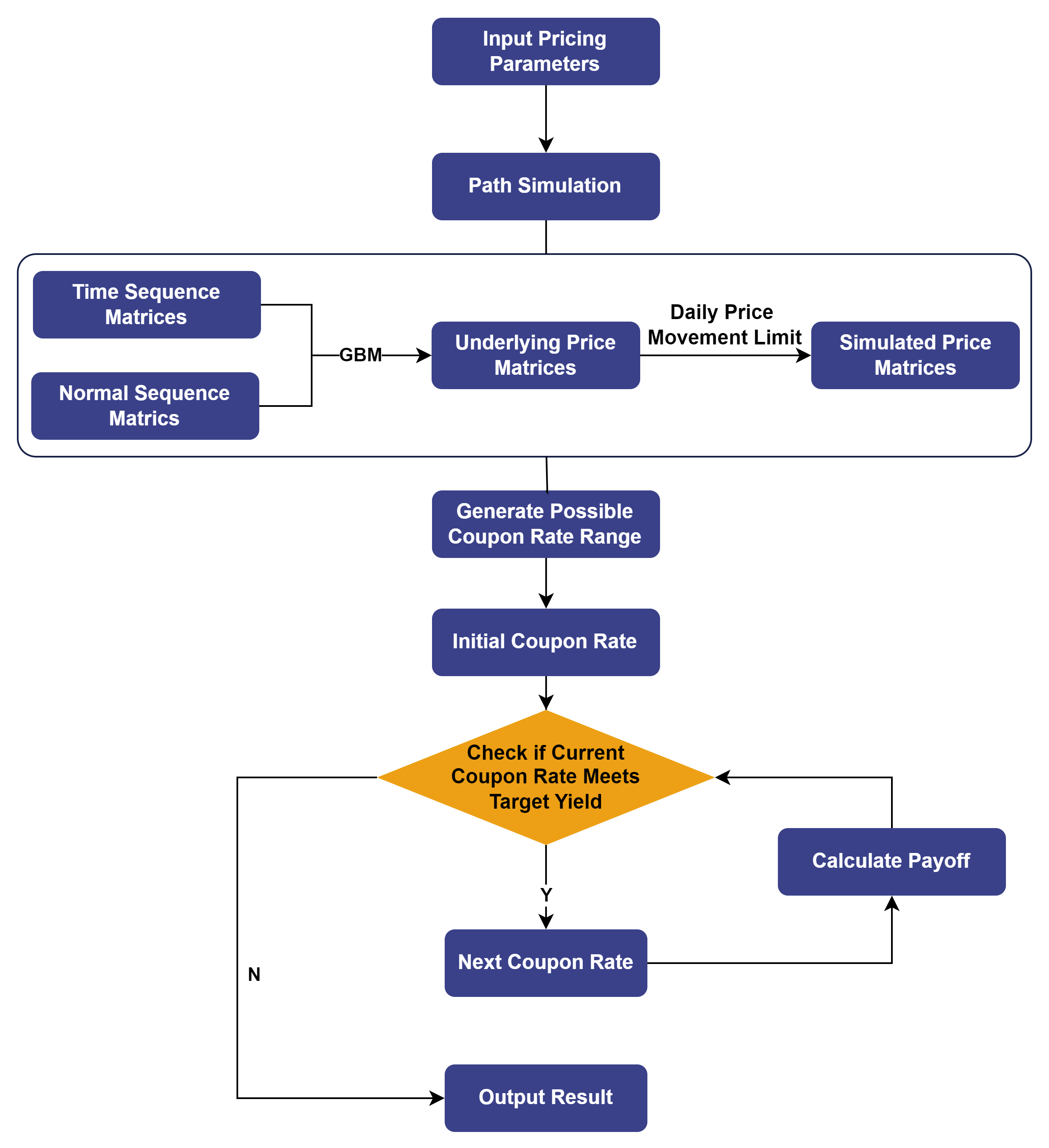
Based on the method described above for determining the coupon rate of a snowball option given a target profit, the logic for calculating the seller’s coupon rate is illustrated below:
3.4.1 Functions for Determining Coupon Rate
Unlike snowball option pricing, determining the coupon rate for a given
target profit requires computing the snowball value using the same simulated
price matrix. Therefore, a dedicated snowball valuation function is defined,
annotated with @gpu to leverage Shark Graph for GPU
acceleration.
@gpu
def calculate_pay_off(coupon, Spath, S, r, T, knock_out_day, knock_in_day, days_in_year){
    // Calculate payoff for three scenarios:
    payoff1 = coupon * knock_out_day / days_in_year * exp(-r * knock_out_day / days_in_year)
    payoff2 = coupon * exp(-r * T)
    payoff3 = (last(Spath) - S)*exp(-r * T)
    // Determine the payoff status for each price path
    payoff = iif(knock_out_day>0, payoff1,
             iif(knock_in_day==0, payoff2,
             iif(last(Spath)<S, payoff3, 0)))
    return payoff
}
An evenly spaced grid search is then applied to generate a range of potential coupon rates at a fixed interval of 0.001. The search continues until the present values corresponding to two adjacent coupon rates bracket the issuer’s target present value.
@gpu
def snowball_pricing(S, r, T, sigma, N, k_out, k_in, lock_period, days_in_year, profit_rate){
    Tdays = T*days_in_year
    monthDay = int(days_in_year/12)
    Spath = simulation(S, r, T, sigma, N, days_in_year) // Simulated price path matrix
    observation_out_idx = monthDay*(1..(Tdays/monthDay))
    observation_out_idx = observation_out_idx[observation_out_idx>lock_period]-1
    knockOutMatrix = Spath[observation_out_idx, ]>=k_out
    knock_out_day = observation_out_idx*knockOutMatrix
    knock_out_day = min(knock_out_day[knock_out_day>0])
    knock_in_day = sum(Spath < k_in)
    knock_out_times = sum(knock_out_day>0) // Number of simulated paths where knock-out occurs
    existence_times = sum(knock_out_day<=0&&knock_in_day==0) // Number of simulated paths with neither knock-in nor knock-out
    knock_in_times = sum(knock_out_day<=0&&knock_in_day>0) // Number of simulated paths with knock-in but no knock-out at expiry
    lose_times = sum(knock_out_day<=0&&knock_in_day>0&&last(Spath)<S) // Number of investor losses (issuer gains)

    // Generate a possible coupon range with fixed intervals
    coupon_test_range = (0..1000)*0.001 // Accurate to four decimal places

    // Search using a for loop
    lastvalue = 0
    lastcoupon = 0
    target = (1-profit_rate)
    for (coupon in coupon_test_range){
        // Calculate the present value for each path
        value = 1.0 + avg(calculate_pay_off(coupon, Spath, S, r, T, knock_out_day, knock_in_day, days_in_year))
        if (value > target > lastvalue){
            break
        }
        lastvalue = value
        lastcoupon = coupon
    }
    // Get the bounds of the interval
    coupon_lower_bound = lastcoupon // Upper bound of coupon
    coupon_upper_bound = coupon // Lower bound of coupon
    return 0.5*(coupon_lower_bound + coupon_upper_bound), knock_out_times, knock_in_times, existence_times, lose_times
}
3.4.2 Function Parameters
The table below lists the parameters used for the function that determines the issuer’s coupon rate. All parameters except profit_rate are the same as those used in the snowball pricing function.
| Parameter & Variable | Description |
|---|---|
| Number of simulated paths (N) | Number of asset price paths simulated using the Monte Carlo method |
| Initial price (S) | Initial price of the underlying asset for the snowball option |
| Trading days per year (days_in_year) | Total number of trading days in a year |
| Lock-up period (lock_period) | Lock-up period (in days) specified by the snowball option contract |
| Knock-in level (k_in) | Knock-in boundary price specified by the snowball option contract |
| Knock-out level (k_out) | Knock-out boundary price specified by the snowball option contract |
| Risk-free rate (r) | User-specified risk-free interest rate |
| Time to maturity (T) | Time to maturity of the snowball option, in years |
| Volatility (sigma) | User-specified annualized volatility of the underlying asset |
| Target profit rate (profit_rate) | Target profit rate for the snowball issuer (issuance cost not considered) |
Parameter configuration and the corresponding execution code are shown below:
N = 300000              // Number of simulated paths
S = 1.0                 // Initial price of the underlying asset
k_in = 0.85             // Knock-in level
k_out = 1.03            // Knock-out level
T = 1                   // Maturity (years)
days_in_year = 252      // Number of trading days in a year
sigma = 0.13            // Annualized volatility of the underlying asset
r = 0.03                // Risk-free rate (annualized)
lock_period = 0         // Lock-up period (days)
profit_rate = 0.01      // Target profit rate for the snowball issuer

timer coupon, knock_out_times, knock_in_times, existence_times, lose_times = snowball_pricing(S, r, T, sigma, N, k_out, k_in, lock_period, days_in_year, profit_rate)
print("Snowball coupon rate:", coupon)
print("Knock-out probability:", knock_out_times \ N)
print("Probability of neither knock-in nor knock-out:", existence_times \ N)
print("Probability of knock-in without knock-out:", knock_in_times \ N)
print("Issuer profit probability:", lose_times \ N) // The issuer’s profit probability equals the buyer’s loss probability
3.4.3 Pricing Results
The output of GPU-accelerated pricing using Shark Graph shows that the coupon rate corresponding to the above parameters is 2.35%.
Time elapsed: 116.619 ms

Snowball coupon rate: 0.0235

Knock-out probability: 0.7385

Probability of neither knock-in nor knock-out: 0.135646666666667

Probability of knock-in without knock-out: 0.125853333333333

Loss probability: 0.12393
4. Performance Testing
4.1 Results
To demonstrate the high-performance computing capability of Shark, we conducted benchmark tests comparing four implementations: DolphinDB Shark (GPU-accelerated), Python, Python with JIT optimization, and R. Each implementation simulated 300,000 underlying price paths for snowball option pricing.
| Software | Version | Snowball Option Pricing Time (ms) | Performance Improvement (×) |
|---|---|---|---|
| DolphinDB Shark | 3.00.3 2025.05.15 LINUX_ABI x86_64 | 36 | \ |
| Python+JIT | 3.12.7 | 1,054 | 29 |
| Python | 3.12.7 | 5,935 | 165 |
| R | 4.5.1 | 19,816 | 550 |
| Software | Version | Snowball Coupon Rate Determination Time (ms) | Performance Improvement (×) |
|---|---|---|---|
| DolphinDB Shark | 3.00.3 2025.05.15 LINUX_ABI x86_64 | 116 | \ |
| Python+JIT | 3.12.7 | 1,213 | 10 |
| Python | 3.12.7 | 6,497 | 56 |
| R | 4.5.1 | 20,518 | 177 |
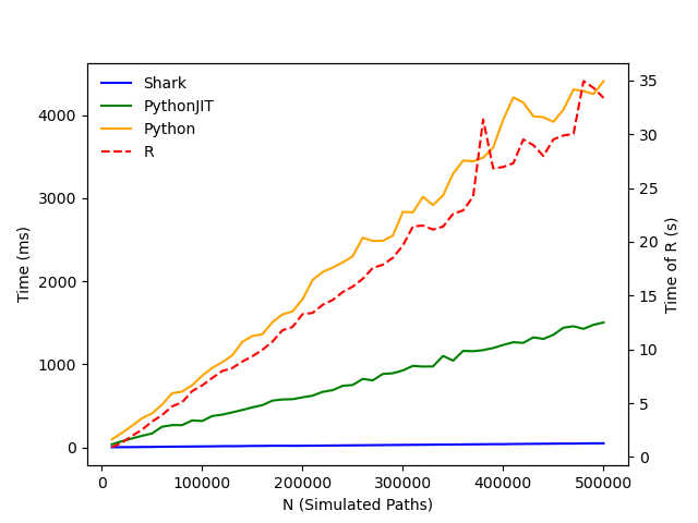
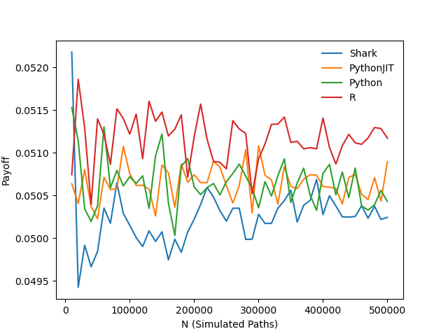
To further evaluate how the number of simulated paths affects pricing accuracy and execution time, we varied the number of Monte Carlo simulation paths from 10,000 to 500,000 in steps of 10,000. For each case, we calculated the snowball option price using the four methods and plotted the execution time (in milliseconds) and the resulting option values.
For coupon rate determination, the same experimental setup was applied: the number of simulated paths was varied from 10,000 to 500,000 in steps of 10,000. Execution time and calculated coupon rates were recorded and visualized for performance comparison.
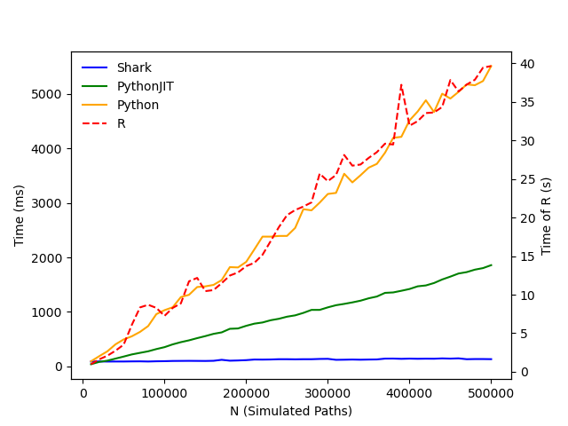
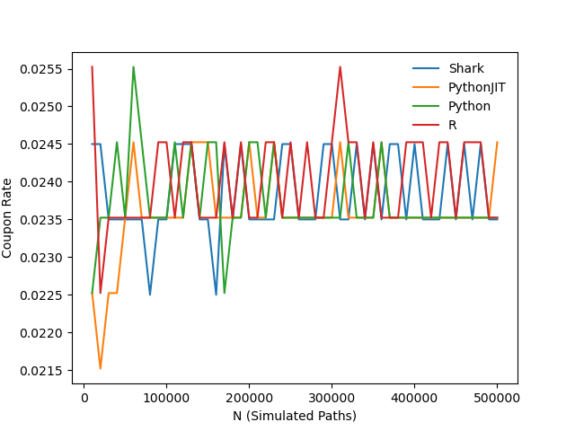
The results show that all four implementations—Shark, Python+JIT, Python, and R—produce consistent pricing and coupon rate outputs, while their execution times differ significantly. Under the test conditions, Shark demonstrated excellent performance, completing snowball option pricing in 36 ms with 500,000 simulated paths and determining the coupon rate for a given target profit in just 116 ms. These results highlight Shark’s high computational efficiency and its strong potential for FICC applications in similar scenarios.
4.2 Test Environment Configuration
DolphinDB is deployed in cluster mode. The hardware and software environments used in this test are as follows:
- Hardware Environment
| Hardware | Configuration Details |
|---|---|
| Kernel | 3.10.0-1160.88.1.el7.x86_64 |
| CPU | Intel(R) Xeon(R) Gold 5220R CPU @ 2.20GHz |
| GPU | NVIDIA A30 24GB (1 unit) |
| Memory | 512GB |
- Software Environment
| Software | Configuration Details |
|---|---|
| Operating System | CentOS Linux 7 (Core) |
| DolphinDB |
Server version: 3.00.3 2025.05.15 LINUX x86_64 License limit: 16 cores, 128 GB |
5. Conclusion
This tutorial demonstrates two key applications—snowball option pricing and coupon rate determination—leveraging the capabilities of Shark Graph on DolphinDB’s CPU-GPU heterogeneous computing platform, Shark. By harnessing DolphinDB’s high-performance computation for practical option pricing scenarios, it highlights DolphinDB’s advantages in FICC applications, enabling faster and more accurate valuation of snowball options.