Quick Start Guide for Shark GPLearn
Overview
GPLearn is often used in quant finance to extract factors from historical data to guide trading decisions for stocks and futures. However, it faces challenges currently:
-
Low performance: To extract high-quality factors, it is necessary to increase the complexity of individual operators, the number of initial formulas, and the number of iterations, which leads to greater computation workloads.
-
Insufficient operators: The basic mathematical operators provided by Python GPLearn are difficult to fit the complex features of financial data.
-
Difficulty in handling 3D data: GPLearn can only handle two-dimensional input data, e.g., data of all stocks at the same time (cross-sectional data) or data of the same stock at different times (time series data). For three-dimensional data (different times + different stocks + features), additional grouping operations (
group by) are required, which increases the complexity of data processing.
Shark GPLearn
Shark GPLearn is a framework designed for solving symbolic regression using genetic algorithms, which aims to automatically generate factors that fit the data distribution. Compared with Python GPLearn, Shark GPLearn brings the following improvements:
-
GPU acceleration: Shark GPLearn utilizes GPUs to significantly improve the efficiency of factor discovery and computation.
-
Extensive operator library: Shark GPLearn integrates the functions built into the DolphinDB database to enrich its operator library, enabling it to accurately fit the complex features of data.
-
Support for 3D data: Shark GPLearn supports the processing of three-dimensional data. Users only need to set the grouping column name for in-group calculation.
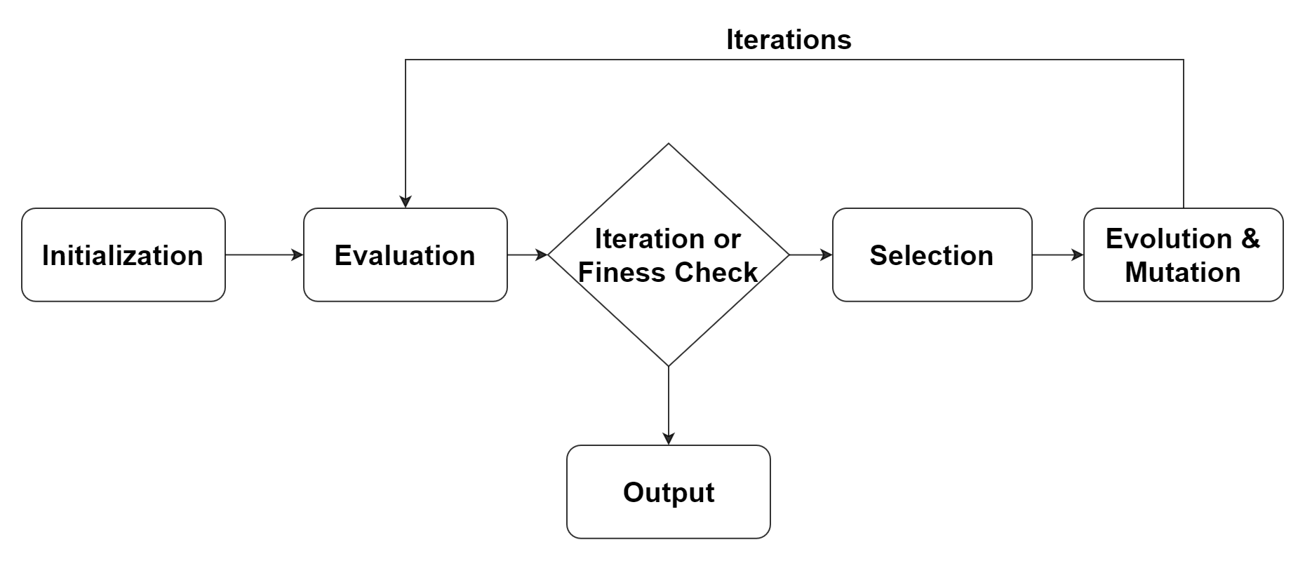
Genetic Programming
A genetic algorithm is a search optimization method inspired by natural selection and Darwin's theory of evolution, especially the idea of "survival of the fittest". There are some key concepts in genetic algorithms, such as "population", "crossover (mating)", "mutation" and "selection", all of which come from the evolutionary theory. A population is the set of all possible solutions. Crossover is a way to generate new solutions by combining parts of two solutions. Mutation is a random change to a solution to increase the diversity of the population. Selection is the process of keeping solutions with better fitness.
The process of genetic programming can be summarized into the following steps:
-
Initialization: Generate a population of random formulas.
-
Evaluation: Evaluate the fitness (i.e., the accuracy of fitting the data) of each formula and give a fitness score.
-
Selection: Select formulas based on their fitness scores for the next generation. Formulas with better fitness scores have a higher probability of being selected.
-
Evolution and mutation: Randomly select two formulas, then exchange part of the formula with the other to generate two new formulas. Or randomly modify a part of the formula to generate a new formula.
-
Iteration: Repeat steps 2-4 until the stopping criterion is met, such as reaching the maximum number of iterations or finding a sufficiently good formula.
Full Example
-
Deploy DolphinDB on a GPU-enabled server.
You must specify libskgraph.so and libshark.so through the dolphinModulePath configuration option. Please set
dolphinModulePath=libskgraph.so,libshark.soin the dolphindb.cfg.Shark GPLearn requires CUDA version >= 12.9 GA and NVIDIA driver version >= 575.51.03, along with your GPU compute capability over 6.0. See NVIDIA Compute Capability for more information.
-
Prepare data for training
def prepareData(num){ total=num data=table(total:total, `a`b`c`d,[FLOAT,FLOAT,FLOAT,FLOAT])// 1024*1024*5 行 data[`a]=rand(10.0, total) - rand(5.0, total) data[`b]=rand(10.0, total) - rand(5.0, total) data[`c]=rand(10.0, total) - rand(5.0, total) data[`d]=rand(10.0, total) - rand(5.0, total) return data } num = 1024 * 1024 * 5 source = prepareData(num) -
Prepare data for prediction
a = source[`a] b = source[`b] c = source[`c] d = source[`d] predVec = a*a*a*a/(a*a*a*a+1) + b*b*b*b/(b*b*b*b+1) + c*c*c*c/( c*c*c*c+1) + d*d*d*d/(d*d*d*d+1) -
Perform training
engine = createGPLearnEngine(source, predVec, functionSet=['add', 'sub', 'mul', 'div', 'sqrt','log', 'abs','neg', 'max','min', 'sin', 'cos', 'tan'], constRange=0,initDepth = [2,5],restrictDepth=true) engine.gpFit(10) -
Make predictions
predict = engine.gpPredict(source, 10) -
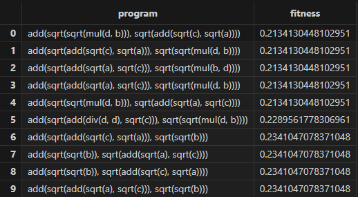
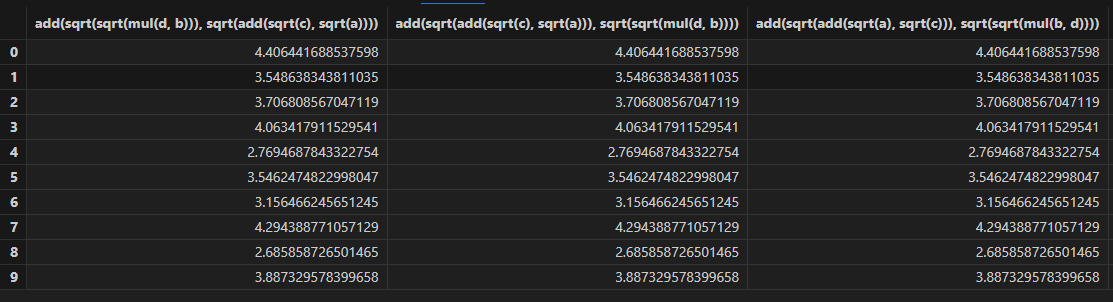
Training output:
- Training process
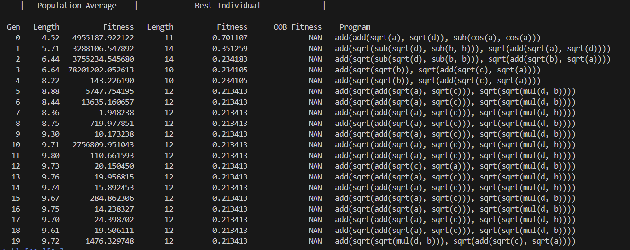
- Training
- Predictions
- Training process
Related Functions
- createGPLearnEngine: Create a GPLearn engine.
- gpFit: Get trained programs.
- gpPredict: Make predictions.
- setGpFitnessFunc: Set fitness function for the GPLearn engine.
- addGpFunction: Add a user-defined training function to the GPLearn engine.
Appendix
The following table lists available functions for building and evolving formulas.
| Function | Description |
|---|---|
| add(x,y) | Addition |
| sub(x,y) | Subtraction |
| mul(x,y) | Multiplication |
| div(x,y) | Division. If the absolute value of the divisor is less than 0.001, returns 1. |
| max(x,y) | Maximum value |
| min(x,y) | Minimum value |
| sqrt(x) | Square root of the absolute value |
| log(x) | Logarithm. If x is less than 0.001, returns 0. |
| neg(x) | Negation |
| reciprocal(x) | Reciprocal. If the absolute value of x is less than 0.001, returns 0. |
| abs(x) | Absolute value |
| sin(x) | Sine function |
| cos(x) | Cosine function |
| tan(x) | Tangent function |
| sig(x) | Sigmoid function |
| signum(x) | Returns the sign of x |
| mcovar(x, y, n) | Covariance of x and y within a sliding window of size n |
| mcorr(x, y, n) | Correlation of x and y within a sliding window of size n |
| mstd(x, n) | Sample standard deviation of x within a sliding window of size n |
| mmax(x, n) | Maximum value of x within a sliding window of size n |
| mmin(x, n) | Minimum value of x within a sliding window of size n |
| msum(x, n) | Sum of x within a sliding window of size n |
| mavg(x, n) | Average of x within a sliding window of size n |
| mprod(x, n) | Product of x within a sliding window of size n |
| mvar(x, n) | Sample variance of x within a sliding window of size n |
| mvarp(x, n) | Population variance of x within a sliding window of size n |
| mstdp(x, n) | Population standard deviation of x within a sliding window of size n |
| mimin(x, n) | Index of the minimum value of x within a sliding window of size n |
| mimax(x, n) | Index of the maximum value of x within a sliding window of size n |
| mbeta(x, y, n) | Least-squares estimate of the regression coefficient of x on y within a window of size n |
| mwsum(x, y, n) | Iner product of x and y within a sliding window of size n |
| mwavg(x, y, n) | Weighted average of x with y as weights within a sliding window of size n |
| mfirst(x,n) | First element of the window of size n |
| mlast(x,n) | Last element of the window of size n |
| mrank(x,asc, n) | Rank of x within the sliding window of size n |
| ratios(x) | Returns the value of x(n)/x(n−1)x(n) / x(n-1) |
| deltas(x) | Returns the value of x(n)−x(n−1)x(n) - x(n-1) |
mmax(x, n)), the
parameter n, which represents the window size, is randomly selected from the
windowRange vector specified in the createGPLearnEngine
function. In the following example, the training process randomly selects a value
from [7,14,21] as the window
size.engine = createGPLearnEngine(source, predVec, windowRange=[7,14,21])