Functional Programming Cases
DolphinDB supports functional programming-a declarative programming style that solves problems by applying a series of functions to data. With higher-order functions, DolphinDB allows functions to be passed as parameters, enhancing code expressiveness, simplifying logic, and enabling complex tasks to be accomplished in just a few lines.
This tutorial explores common use cases of functional programming in DolphinDB, with a focus on higher-order functions and their applications.
1. Data Import Use Cases
In many CSV files, time is represented as integers — for example,
93100000 corresponds to “9:31:00.000”. To make querying and
analysis more convenient, it’s recommended to convert such values into the
TIME data type before storing them in a DolphinDB database.
To handle this, the loadTextEx function's transform parameter
can be used to specify how to convert the time column during data import.
1.1 Converting Integer Timestamps to TIME Type
In the following example, we’ll use a sample CSV file named candle_201801.csv, with data like the following:
symbol,exchange,cycle,tradingDay,date,time,open,high,low,close,volume,turnover,unixTime
000001,SZSE,1,20180102,20180102,93100000,13.35,13.39,13.35,13.38,2003635,26785576.72,1514856660000
000001,SZSE,1,20180102,20180102,93200000,13.37,13.38,13.33,13.33,867181
......(1)Create the Database
Create a database VALUE partitioned on dates:
login(`admin,`123456)
dataFilePath="/home/data/candle_201801.csv"
dbPath="dfs://DolphinDBdatabase"
db=database(dbPath,VALUE,2018.01.02..2018.01.30)(2)Create the Table
First, use the extractTextSchema function to infer the table
schema from the CSV file. The “time” column is recognized as INT type. To store
it as TIME, use an UPDATE statement to change its type in the schema, and then
use this modified schema to create a partitioned table (partitioned by the
“date” column).
schemaTB=extractTextSchema(dataFilePath)
update schemaTB set type="TIME" where name="time"
tb=table(1:0, schemaTB.name, schemaTB.type)
tb=db.createPartitionedTable(tb, `tb1, `date);Note: Instead of using extractTextSchema, you may also
define the schema manually.
(3) Importing the Data
First define a transformation function i2t to preprocess the
“time” column, converting it from INT to TIME type. This function is then passed
to loadTextEx using the transform parameter so the
conversion happens automatically during import.
def i2t(mutable t){
    return t.replaceColumn!(`time, t.time.format("000000000").temporalParse("HHmmssSSS"))
}Note: When modifying data inside a function, use in-place operations
(functions ending with !) to boost performance.
Import the data using:
tmpTB=loadTextEx(dbHandle=db, tableName=`tb1, partitionColumns=`date, filename=dataFilePath, transform=i2t);(4) Querying the data
To verify the results, check the first two rows:
select top 2 * from loadTable(dbPath,`tb1);

symbol exchange cycle tradingDay date       time               open  high  low   close volume  turnover   unixTime
------ -------- ----- ---------- ---------- --------------     ----- ----- ----- ----- ------- ---------- -------------
000001 SZSE     1     2018.01.02 2018.01.02 09:31:00.000       13.35 13.39 13.35 13.38 2003635 2.678558E7 1514856660000
000001 SZSE     1     2018.01.02 2018.01.02 09:32:00.000       13.37 13.38 13.33 13.33 867181  1.158757E7 1514856720000
Complete Code
login(`admin,`123456)
dataFilePath="/home/data/candle_201801.csv"
dbPath="dfs://DolphinDBdatabase"
db=database(dbPath,VALUE,2018.01.02..2018.01.30)
schemaTB=extractTextSchema(dataFilePath)
update schemaTB set type="TIME" where name="time"
tb=table(1:0,schemaTB.name,schemaTB.type)
tb=db.createPartitionedTable(tb,`tb1,`date);

def i2t(mutable t){
    return t.replaceColumn!(`time,t.time.format("000000000").temporalParse("HHmmssSSS"))
}

tmpTB=loadTextEx(dbHandle=db,tableName=`tb1,partitionColumns=`date,filename=dataFilePath,transform=i2t);
1.2 Converting Integer Timestamps to NANOTIMESTAMP Type
In this example, we'll import data where nanosecond timestamps are stored as integers, and convert them into the NANOTIMESTAMP type. The example uses a text file named nx.txt, with sample data like this:
SendingTimeInNano#securityID#origSendingTimeInNano#bidSize
1579510735948574000#27522#1575277200049000000#1
1579510735948606000#27522#1575277200049000000#2
...
Each line uses # as the delimiter. The “SendingTimeInNano” and
“origSendingTimeInNano” columns contain timestamps in nanosecond format.
(1) Creating the Database and Table
We start by defining a COMPO-partitioned DFS database db, and table nx with specified column names and types:
dbSendingTimeInNano = database(, VALUE, 2020.01.20..2020.02.22);
dbSecurityIDRange = database(, RANGE,  0..10001);
db = database("dfs://testdb", COMPO, [dbSendingTimeInNano, dbSecurityIDRange]);

nameCol = `SendingTimeInNano`securityID`origSendingTimeInNano`bidSize;
typeCol = [`NANOTIMESTAMP,`INT,`NANOTIMESTAMP,`INT];
schemaTb = table(1:0,nameCol,typeCol);

db = database("dfs://testdb");
nx = db.createPartitionedTable(schemaTb, `nx, `SendingTimeInNano`securityID);
(2) Importing the Data
To import the data, we define a transformation function that converts integer
timestamps into the NANOTIMESTAMP type using the nanotimestamp
function:
def dataTransform(mutable t){
  return t.replaceColumn!(`SendingTimeInNano, nanotimestamp(t.SendingTimeInNano)).replaceColumn!(`origSendingTimeInNano, nanotimestamp(t.origSendingTimeInNano))
}
Finally, we use loadTextEx to import the data.
Complete Code
dbSendingTimeInNano = database(, VALUE, 2020.01.20..2020.02.22);
dbSecurityIDRange = database(, RANGE,  0..10001);
db = database("dfs://testdb", COMPO, [dbSendingTimeInNano, dbSecurityIDRange]);

nameCol = `SendingTimeInNano`securityID`origSendingTimeInNano`bidSize;
typeCol = [`NANOTIMESTAMP,`INT,`NANOTIMESTAMP,`INT];
schemaTb = table(1:0,nameCol,typeCol);

db = database("dfs://testdb");
nx = db.createPartitionedTable(schemaTb, `nx, `SendingTimeInNano`securityID);

def dataTransform(mutable t){
  return t.replaceColumn!(`SendingTimeInNano, nanotimestamp(t.SendingTimeInNano)).replaceColumn!(`origSendingTimeInNano, nanotimestamp(t.origSendingTimeInNano))
}

pt=loadTextEx(dbHandle=db,tableName=`nx , partitionColumns=`SendingTimeInNano`securityID,filename="nx.txt",delimiter='#',transform=dataTransform);
For more on text file importing, see user manual.
2. Lambda Expressions
In DolphinDB, you can define two types of functions: named functions and anonymous functions. Anonymous functions are often implemented as lambda expressions, which are concise function definitions containing just a single statement.
The following example uses the lambda expression x -> x + 1 as the
input function for the each operation:
x = 1..10
each(x -> x + 1, x)
This lambda expression takes a value x and returns x + 1. When used
with the each function, it applies this operation to every element
in the vector 1 to 10.
Additional examples of lambda expressions will be introduced in the following chapters.
3. Use Cases of Higher-order Functions
3.1 cross (:C)
3.1.1 Applying a Function Pairwise to Two Vectors or Matrices
The cross function allows you to apply a binary function to
the permutation of all individual elements from two input vectors or
matrices. The pseudocode is as follows:
for(i:0~(size(X)-1)){
   for(j:0~(size(Y)-1)){
       result[i,j]=<function>(X[i], Y[j]);
   }
}
return result;
For example, computing a covariance matrix traditionally requires nested
for loops, as shown below:
def matlab_cov(mutable matt){
	nullFill!(matt,0.0)
	rowss,colss=matt.shape()
	msize = min(rowss, colss)
	df=matrix(float,msize,msize)
	for (r in 0..(msize-1)){
		for (c in 0..(msize-1)){
			df[r,c]=covar(matt[:,r],matt[:,c])
		}
	}
	return df
}
While the logic here is straightforward, the code is verbose, harder to maintain, and more error-prone.
In DolphinDB, you can use the higher-order function cross
(or pcross for parallel computing) to achieve the same
result in a much simpler way:
cross(covar, matt)3.2 each (:E)
In some scenarios, we may need to apply a function to every element within a
given parameter. Without functional programming, this often requires a
for loop. DolphinDB offers higher-order functions such as
each, peach, loop, and
ploop, which simplify the code significantly.
3.2.1 Counting NULL Values in Each Column
In DolphinDB:
sizereturns the total number of elements in a vector or matrix.countreturns only the number of non-NULL elements.
Therefore, the difference between size and
count gives the number of NULLs. For tables, we can
efficiently count NULL values in each column using the higher-order function
each:
each(x->x.size() - x.count(), t.values())This works because t.values() returns a tuple containing all
columns of table t, and the lambda expression x->x.size() -
x.count() calculates the NULL count for each column.
3.2.2 Removing Rows Containing NULL values
Let's start by creating a sample table with some NULL values:
sym = take(`a`b`c, 110)
id = 1..100 join take(int(),10)
id2 =  take(int(),10) join 1..100
t = table(sym, id,id2)
There are two ways to remove rows with NULL values.
Method 1: Row-wise Filtering
This approach checks each row individually:
t[each(x -> !(x.id == NULL || x.id2 == NULL), t)]Note that for row operations on tables, each row is represented as a dictionary. In this example expression, the lambda expression checks for NULL values in the specified columns id and id2.
If the table has many columns and listing each one is impractical, use this expression instead:
t[each(x -> all(isValid(x.values())), t)]This works by:
- Getting all values in a row as a dictionary with
x.values() - Checking for valid (non-NULL) values with
isValid()in each row - Using
all()to ensure every value in the row is valid
However, when working with large datasets, row-wise operations can be inefficient.
Method 2: Column-wise Filtering for Better Performance
Since DolphinDB uses columnar storage, column operations typically outperform row operations. We can leverage this with:
t[each(isValid, t.values()).rowAnd()]Use each with isValid to apply the function
to each column and get the result in a matrix. Then use
rowAnd to identify rows without NULLs:
For extremely large datasets that might trigger the error:
The number of cells in a matrix can't exceed 2 billions.Use reduce to perform iterative column-wise validation:
t[reduce(def(x,y) -> x and isValid(y), t.values(), true)]3.2.3 Performance Comparison: Row-wise vs Column-wise Processing
The following example demonstrates how to transform a column in a table by changing "aaaa_bbbb" to "bbbb_aaaa".
First, create a table t:
t=table(take("aaaa_bbbb", 1000000) as str);There are two approaches to perform this transformation: row-wise and column-wise processing.
Row-wise Processing: Use the higher-order function
each to iterate through each row, splitting the string
and reversing the segments:
each(x -> split(x, '_').reverse().concat('_'), t[`str])Column-wise Processing: Locate the position of the underscore and then use string operations on the entire column:
pos = strpos(t[`str], "_")
substr(t[`str], pos+1)+"_"+t[`str].left(pos)
When comparing performance between the two approaches, row-wise processing requires approximately 2.3 seconds to complete, while column-wise processing executes significantly faster at just 100 milliseconds.
Complete Code
t=table(take("aaaa_bbbb", 1000000) as str);

timer r = each(x -> split(x, '_').reverse().concat('_'), t[`str])

timer {
	pos = strpos(t[`str], "_")
	r = substr(t[`str], pos+1)+"_"+t[`str].left(pos)
}
3.2.4 Checking if Two Tables are Identical
To determine whether two tables contain exactly the same data, use the
higher-order function each to compare each column in both
tables. For example, for tables t1 and t2:
all(each(eqObj, t1.values(), t2.values()))3.3 loop (:U)
The higher-order functions loop and each are
similar, but they differ in the format and type of their return values.
The each function determines the data form of its return based
on the type and form of the result from each subtask:
- If each subtask returns a scalar,
eachreturns a vector. - If each subtask returns a vector,
eachreturns a matrix. - If each subtask returns a dictionary,
eachreturns a table. - If the return types or forms of the subtasks vary,
eachreturns a tuple; otherwise, it returns a vector or matrix as appropriate.
For example:
m=1..12$4:3;
m;
each(add{1 2 3 4}, m);
This yields:
| col1 | col2 | col3 |
|---|---|---|
| 2 | 6 | 10 |
| 4 | 8 | 12 |
| 6 | 10 | 14 |
| 8 | 12 | 16 |
On the other hand, loop always returns a tuple. For instance, to
calculate the maximum value of each column:
t = table(1 2 3 as id, 4 5 6 as value, `IBM`MSFT`GOOG as name);
t;
loop(max, t.values());
This yields:
| offset | 0 | 1 | 2 |
|---|---|---|---|
| 0 | 3 | 6 | MSFT |
Importing multiple files
Suppose we have multiple CSV files with the same structure stored in a directory,
and we want to import them into a single in-memory table in DolphinDB. We can
use loop to achieve this:
loop(loadText, fileDir + "/" + files(fileDir).filename).unionAll(false)3.4 moving / rolling
3.4.1 moving
This example shows how to use the moving function to
determine whether the values of a column fall within a specified range.
For each record, use the columns “UpAvgPrice” and “DownAvgPrice” to define a range. Then we look at the previous 20 values of the “close” column and check whether they fall within the range [DownAvgPrice, UpAvgPrice]. If at least 75% of those values are within the range, the “signal” column is set to true; otherwise, it's false.
Sample Data:
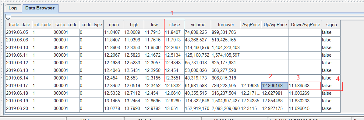
For instance, for the record where “trade_date” is 2019.06.17, the range is [11.5886533, 12.8061868]. We examine the 20 preceding “close” values (column marked as "1" in the figure). If at least 75% fall within the range, the corresponding “signal” value (column "4") is set to true.
Solution:
We define a function rangeTest that checks whether the
percentage of “close” values in a given window fall within the specified
range [DownAvgPrice, UpAvgPrice]. Then use the higher-order function
moving to apply rangeTest to each
sliding window in the dataset.
defg rangeTest(close, downlimit, uplimit){
  size = close.size() - 1
  return between(close.subarray(0:size), downlimit.last():uplimit.last()).sum() >= size*0.75
}

update t set signal = moving(rangeTest, [close, downAvgPrice, upAvgPrice], 21)
In this example:
- Since we're checking the 20 rows before the current one, the window size is set to 21 (20 previous + current row).
- The
betweenfunction is used to check whether each value falls within the inclusive range defined by a and b.
We can simulate real market data to validate the script above. For example:
t=table(rand("d"+string(1..n),n) as ts_code, nanotimestamp(2008.01.10+1..n) as trade_date, rand(n,n) as open, rand(n,n) as high, rand(n,n) as low, rand(n,n) as close, rand(n,n) as pre_close, rand(n,n) as change, rand(n,n) as pct_chg, rand(n,n) as vol, rand(n,n) as amount, rand(n,n) as downAvgPrice, rand(n,n) as upAvgPrice, rand(1 0,n) as singna)Note on rolling vs
moving
Both rolling and moving apply a function to
a sliding window over a dataset. However, there are some key
differences:
rollingallows you to set a custom step size (step), whilemovingalways uses a step of 1.- Their behavior in handling null values differs. For more information, refer to the Window Calculations.
3.4.2 Performance Comparison: moving(sum) vs
msum
Although DolphinDB provides the moving higher-order
function, for performance-critical operations, it’s recommended to use
specialized m- functions (such as msum,
mcount, mavg, etc.) whenever
possible.
Example:
x=1..1000000
timer moving(sum, x, 10)
timer msum(x, 10)
Depending on data size, msum can be 50 to 200 times faster
than moving(sum).
Why the performance difference?
- Data access:
msumloads data into memory once and reuses it;moving(sum)creates a new sub-object for each window, which involves memory allocation and cleanup. - Computation method:
msumuses incremental computation — it reuses the previous result by adding the new value and subtracting the value that falls out of the window. In contrast,moving(sum)recalculates the entire window each time.
3.5 eachPre (:P)
In this case, we first create a table t with two columns: sym and bidPrice:
t = table(take(`a`b`c`d`e ,100) as sym, rand(100.0,100) as bidPrice)We want to perform the following calculations:
- Compute a new column “ln”: This column stores the result of the following calculation: For each row, divide the current bidPrice by the average bidPrice of the previous 3 rows (excluding the current row), and then take the natural logarithm of the result.
- Compute a new column “clean” based on “ln”: This column filters out
abnormal values in “ln”. The logic is:
- Take the absolute value of “ln”.
- If it exceeds a fluctuation threshold F, then use the previous “ln” value instead. Otherwise, treat the current value as normal and keep it.
Since the computation of “ln“ involves a sliding window of size 3, we can refer to the example in section 3.4.1. The corresponding script is:
t2 = select *, log(bidPrice / prev(moving(avg, bidPrice,3))) as ln from tHowever, for better performance, we can use built-in function
mavg, which is more efficient than the
moving higher-order function. The code can be rewritten in
two equivalent ways:
//method 1
t2 = select *, log(bidPrice / prev(mavg(bidPrice,3))) as ln from t

//method 2
t22 = select *, log(bidPrice / mavg(prev(bidPrice),3)) as ln from t
Here, prev returns the data from the previous row.
Both approaches give equivalent results. The only difference is that in t22, a value is generated starting from the third row.
Now, to clean abnormal values in “ln”. Assuming the fluctuation threshold
F is 0.02, we define a function cleanFun as follows:
F = 0.02
def cleanFun(F, x, y): iif(abs(x) > F, y, x)- x is the current “ln” value.
- y is the previous “ln” value.
- If the absolute value of x exceeds F, the function returns y instead of x.
Then we use the high-order function eachPre to apply this logic
pairwise across the column. The implementation of eachPre is
equivalent to: F(X[0], pre), F(X[1], X[0]), ..., F(X[n], X[n-1]). The
corresponding code:
t2[`clean] = eachPre(cleanFun{F}, t2[`ln])Here is the complete script:
F = 0.02
t = table(take(`a`b`c`d`e ,100) as sym, rand(100.0,100) as bidPrice)
t2 = select *, log(bidPrice / prev(mavg(bidPrice,3))) as ln from t
def cleanFun(F,x,y) : iif(abs(x) > F, y,x)
t2[`clean] = eachPre(cleanFun{F}, t2[`ln])
3.6 byRow (:H)
This example demonstrates how to find the index of the maximum value in each row of a matrix. First, we define a matrix m as follows:
a1 = 2 3 4
a2 = 1 2 3
a3 = 1 4 5
a4 = 5 3 2
m = matrix(a1,a2,a3,a4)
One approach is to calculate the index of the maximum value for each row
individually. This can be done using the imax function. By
default, imax operates on each column of a matrix and returns a
vector.
To compute the result by row instead, we can first transpose the matrix and then
apply imax:
imax(m.transpose())Alternatively, DolphinDB provides a higher-order function byRow,
which applies a specified function to each row of a matrix. This avoids the need
to transpose the matrix:
byRow(imax, m)The same operation can also be performed using the built-in row function
rowImax:
print rowImax(m)3.7 segmentby
The segmentby function is a higher-order function used to apply
a computation to segments of data, where each segment is defined by consecutive
identical values in another vector. The high-order function
segmentby has the following syntax:
segmentby(func, funcArgs, segment)func specifies the operation to perform on each segment, funcArgs provides the data to be processed, and segment determines how the data is divided into groups. When consecutive elements in segment have the same value, they form a single group. Each group of values from funcArgs is processed independently by func, and the results are combined to produce an output vector with the same length as the original segment vector.
x = 1 2 3 0 3 2 1 4 5
y = 1 1 1 -1 -1 -1 1 1 1
segmentby(cumsum, x, y)
In the above example, y defines three groups: 1 1 1, -1 -1 -1, and 1 1 1.
Based on this grouping, x is divided accordingly into: 1 2 3, 0 3 2, and
1 4 5. The cumsum function is then applied to each group of x,
computing the cumulative sum within each segment.
DolphinDB also provides the built-in segment function, which is
used for grouping in SQL queries. Unlike segmentby, it only
returns group identifiers without performing calculations.
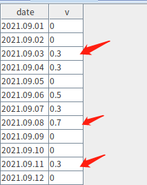
The following example shows how to group data based on a threshold value. Continuous values that are either above or below the threshold are grouped together. For groups where values exceed the threshold, we retain only the record with the maximum value within each group (if there are duplicates, only the first is kept).
Given the table below, when the threshold is set to 0.3,the rows indicated by arrows should be kept:
Define the table:
dated = 2021.09.01..2021.09.12
v = 0 0 0.3 0.3 0 0.5 0.3 0.7 0 0 0.3 0
t = table(dated as date, v)
To group the data based on whether values are continuously greater than minV, use
the segment function:
segment(v >= minV)In SQL, we can combine segment with the CONTEXT BY clause to
perform group calculations. Then, filter for groups with the maximum value using
the HAVING clause. Since filtering might return multiple rows, use the LIMIT
clause to keep only the first matching record per group.
Here is the complete SQL query:
select * from t
context by segment(v >= minV)
having (v = max(v) and v >= minV)
limit 1
3.8 pivot
The high-order function pivot reorganizes data along two
specified dimensions and returns the result as a matrix.
Suppose we have a table t1 with four columns:
syms=`600300`600400`600500$SYMBOL
sym=syms[0 0 0 0 0 0 0 1 1 1 1 1 1 1 2 2 2 2 2 2 2]
time=09:40:00+1 30 65 90 130 185 195 10 40 90 140 160 190 200 5 45 80 140 170 190 210
price=172.12 170.32 172.25 172.55 175.1 174.85 174.5 36.45 36.15 36.3 35.9 36.5 37.15 36.9 40.1 40.2 40.25 40.15 40.1 40.05 39.95
volume=100 * 10 3 7 8 25 6 10 4 5 1 2 8 6 10 2 2 5 5 4 4 3
t1=table(sym, time, price, volume);
t1;
We want to reorganize the data in t1 by the columns “time” (at the minute level) and “sym”, and compute the volume-weighted average price (VWAP) for each stock per minute.
To do this, we use the pivot function:
stockprice = pivot(wavg, [t1.price, t1.volume], minute(t1.time), t1.sym)
stockprice.round(2)
3.9 contextby (:X)
The higher-order function contextby groups data based on
specified column(s) and applies a given function within each group.
Example:
sym = `IBM`IBM`IBM`MS`MS`MS
price = 172.12 170.32 175.25 26.46 31.45 29.43
qty = 5800 700 9000 6300 2100 5300
trade_date = 2013.05.08 2013.05.06 2013.05.07 2013.05.08 2013.05.06 2013.05.07
contextby(avg, price, sym)
The contextby function can also be used in SQL queries. For
example, the following query uses contextby to select trades
where the price is above the group average:
t1 = table(trade_date, sym, qty, price)
select trade_date, sym, qty, price from t1 where price > contextby(avg, price, sym)
3.10 call / unifiedCall
When we need to apply different functions to the same set of inputs in batch, we
can use the higher-order functions
call/unifiedCall together with
each/ loop.
call and unifiedCall
serve the same purpose but differ in how they accept parameters. For details,
refer to function reference.In the example below, the call function is used within a partial
application to apply the functions sin and log
to a fixed vector [1, 2, 3] using the higher-order function
each:
each(call{, 1..3}, (sin, log));Functions can also be invoked dynamically using metaprogramming with
funcByName. The previous example can be rewritten as:
each(call{, 1..3}, (funcByName("sin"), funcByName("log")));funcByName. In
real-world applications, funcByName enables dynamic passing of
functions at runtime.You can also use makeCall or
makeUnifiedCall to generate executable code
representations of function calls, which can then be evaluated (using
eval)
later:
each(eval, each(makeCall{, 1..3}, (sin, log)));3.11 accumulate (:A)
Given minute-level trading data, the goal is to split the data for a stock into segments such that each segment contains approximately 1.5 million shares traded. The length of each time window will vary depending on how many trading records are needed to reach this volume. The rule for segmentation is: if adding the current data point brings the total volume closer to the 1.5 million share target, include it in the current segment; otherwise, begin a new segment starting from that point.
Generate a sample dataset:
timex = 13:03:00+(0..27)*60
volume = 288658 234804 182714 371986 265882 174778 153657 201388 175937 138388 169086 203013 261230 398871 692212 494300 581400 348160 250354 220064 218116 458865 673619 477386 454563 622870 458177 880992
t = table(timex as time, volume)
We define a grouping function to accumulate volume and split segments when the cumulative volume gets closest to 1.5 million:
def caclCumVol(target, preResult, x){
 result = preResult + x
 if(result - target> target - preResult) return x
 else return result
}
accumulate(caclCumVol{1500000}, volume)
caclCumVol accumulates the volume values and segments the data
when the cumulative sum approaches 1.5 million most closely. A new group starts
from the next value.
To identify the start of each group, we compare the accumulated volume with the
original volume values. If they are equal, that point marks the start of a new
group. We then use ffill() to forward-fill these start
times:
iif(accumulate(caclCumVol{1500000}, volume) == volume, timex, NULL).ffill()Finally, we group the data by these start times and perform aggregations.
output = select
    sum(volume) as sum_volume,
    last(time) as endTime
from t
group by iif(accumulate(caclCumVol{1500000}, volume) == volume, time, NULL).ffill() as startTime
Complete Script:
timex = 13:03:00+(0..27)*60
volume = 288658 234804 182714 371986 265882 174778 153657 201388 175937 138388 169086 203013 261230 398871 692212 494300 581400 348160 250354 220064 218116 458865 673619 477386 454563 622870 458177 880992
t = table(timex as time, volume)

def caclCumVol(target, preResult, x){
 result = preResult + x
 if(result - target> target - preResult) return x
 else return result
}
output = select sum(volume) as sum_volume, last(time) as endTime from t group by iif(accumulate(caclCumVol{1500000}, volume)==volume, time, NULL).ffill() as startTime
3.12 window
This example demonstrates how to use the window function to
process a column in a table. The goal is to determine whether a given value is
the minimum within both its preceding 5 values and following 5 values (both
including itself). If it is, mark it as 1; otherwise, mark it as 0.
First, create a table t:
t = table(rand(1..100,20) as id)Next, apply the window function to define a sliding window of 9
elements centered on each row (4 before, the current one, and 4 after). Within
this window, use the min function to find the minimum value.
Note: The window function includes the boundary values in the
window range.
The implementation is as follows:
select *, iif(id==window(min, id, -4:4), 1, 0) as mid from t3.13 reduce (:T)
Some of the previous examples also made use of the higher-order function
reduce. Here's the pseudocode for it:
result = <function>(init, X[0])
for (i = 1 to size(X) - 1) {
  result = <function>(result, X[i])
}
return result
Unlike accumulate, which returns all intermediate results,
reduce only returns the final result.
For example, in the following factorial calculation:
r1 = reduce(mul, 1..10)
r2 = accumulate(mul, 1..10)[9]
Both r1 and r2 produce the same final result.
4. Partial Application Use Cases
Partial application is a technique where some of a function’s arguments are fixed in advance, creating a new function that takes fewer parameters. It’s especially useful with higher-order functions that expect functions with a specific number of arguments.
4.1 Scheduling a Parameterized Job
Suppose we need to set up a scheduled job that runs daily at midnight to calculate the maximum temperature recorded by a specific device on the previous day.
Assume that the temperature data is stored in a table named “sensor” located in
the distributed database dfs://dolphindb. The table contains a timestamp column
ts of type DATETIME. The following script defines a function
getMaxTemperature to perform the required calculation:
def getMaxTemperature(deviceID){
    maxTemp=exec max(temperature) from loadTable("dfs://dolphindb","sensor")
            where ID=deviceID ,date(ts) = today()-1
    return  maxTemp
}
Once the function is defined, we can use the scheduleJob
function to submit the scheduled job. However, since
scheduleJob does not allow passing arguments to the job
function directly—and getMaxTemperature requires the
deviceID as a parameter—we can use partial application to bind the
argument in advance, effectively turning it into a no-argument function:
scheduleJob(`testJob, "getMaxTemperature", getMaxTemperature{1}, 00:00m, today(), today()+30, 'D');This example schedules the job to calculate the maximum temperature for device ID 1.
The complete script looks like this:
def getMaxTemperature(deviceID){
    maxTemp=exec max(temperature) from loadTable("dfs://dolphindb","sensor")
            where ID=deviceID ,date(ts) = today()-1
    return  maxTemp
}

scheduleJob(`testJob, "getMaxTemperature", getMaxTemperature{1}, 00:00m, today(), today()+30, 'D');
4.2 Retrieving Job Information from Other Nodes
In DolphinDB, after submitting scheduled jobs, we can use the
getRecentJobs function to check the status of recent batch
jobs (including scheduled jobs) on the local node. For example, to view the
statuses of the three most recent batch jobs on the local node, use the
following script:
getRecentJobs(3);To retrieve job information from other nodes in the cluster, use the
rpc function to call getRecentJobs on the
remote node. For example, to get job information from the node with the alias
P1-node1, we can do the following:
rpc("P1-node1",getRecentJobs)However, if we try to retrieve the three most recent jobs from
P1-node1 using the following script, it will result in an
error:
rpc("P1-node1",getRecentJobs(3))This is because the second argument of the rpc function must be
a function (either built-in or user-defined), not the result of a function call.
To work around this, we can use partial application to bind the argument to
getRecentJobs, creating a new function that can be passed
to rpc:
rpc("P1-node1",getRecentJobs{3})4.3 Using Stateful Functions in Stream Computing
In stream computing, users typically need to define a message processing function that handles incoming messages. This function generally accepts a single argument (the incoming subscription data) or a table, making it challenging to maintain state between processing events.
However, partial application offers a solution to this limitation. The following
example uses partial application to define a stateful message handler called
cumulativeAverage, which calculates the cumulative average
of incoming data.
We first define a stream table trades. For each incoming message, we calculate the average of the price column and output the result to the avgTable. Here's the script:
share streamTable(10000:0,`time`symbol`price, [TIMESTAMP,SYMBOL,DOUBLE]) as trades
avgT=table(10000:0,[`avg_price],[DOUBLE])

def cumulativeAverage(mutable avgTable, mutable stat, trade){
   newVals = exec price from trade;

   for(val in newVals) {
      stat[0] = (stat[0] * stat[1] + val )/(stat[1] + 1)
      stat[1] += 1
      insert into avgTable values(stat[0])
   }
}

subscribeTable(tableName="trades", actionName="action30", handler=cumulativeAverage{avgT,0.0 0.0}, msgAsTable=true)
In the user-defined function cumulativeAverage, avgTable
is the output table that stores the results. stat is a vector holding
two values: stat[0] stores the current cumulative average, and
stat[1] keeps track of the count of processed values. The
function updates these values as it processes each message and inserts the
updated average into the output table.
When subscribing to the stream table, we use partial application to pre-bind the first two parameters (avgTable and stat), allowing us to create a “stateful” function.
5. Financial Use Cases
5.1 Downsampling Tick Data Using MapReduce
The following example demonstrates how to use the mr (MapReduce) function to convert
high-frequency tick data into minute-level data.
In DolphinDB, we can use a SQL query to aggregate tick data into minute-level data:
minuteQuotes = select avg(bid) as bid, avg(ofr) as ofr from t group by symbol, date, minute(time) as minuteThis can also be achieved using DolphinDB’s distributed computing framework. The
mr (MapReduce) function is a core feature of DolphinDB’s
distributed computing framework.
Here is the full script:
login(`admin, `123456)
db = database("dfs://TAQ")
quotes = db.loadTable("quotes")

//create a new table quotes_minute
model=select  top 1 symbol,date, minute(time) as minute,bid,ofr from quotes where date=2007.08.01,symbol=`EBAY
if(existsTable("dfs://TAQ", "quotes_minute"))
db.dropTable("quotes_minute")
db.createPartitionedTable(model, "quotes_minute", `date`symbol)

//populate data for table quotes_minute
def saveMinuteQuote(t){
minuteQuotes=select avg(bid) as bid, avg(ofr) as ofr from t group by symbol,date,minute(time) as minute
loadTable("dfs://TAQ", "quotes_minute").append!(minuteQuotes)
return minuteQuotes.size()
}

ds = sqlDS(<select symbol,date,time,bid,ofr from quotes where date between 2007.08.01 : 2007.08.31>)
timer mr(ds, saveMinuteQuote, +)
5.2 Data Replay and High-Frequency Factor Calculation
Stateful factors rely not only on current data but also on historical data for their calculations. Calculating such factors generally involves the following steps:
- Save the current batch of incoming messages.
- Compute the factor using the updated historical data.
- Write the computed factor to an output table.
- Optionally, clean up historical data that will no longer be needed.
In DolphinDB, message processing functions must be unary—they can only take the current message as input. To preserve historical state and still compute factors within the message handler, partial application is used. This technique fixes some parameters (to store state) and leaves one open for incoming messages. These fixed parameters are contained only within that specific message handler function.
The historical state can be stored in in-memory tables, dictionaries, or in-memory partitioned tables. This example uses a dictionary to store quote data and compute a factor using DolphinDB's streaming engines. For implementations using memory or in-memory partitioned tables, refer to Calculating High Frequency Factors in Real-Time.
Defining the Factor: We define a factor that calculates the ratio between the current ask price (askPrice1) and the ask price from 30 quotes ago.
The corresponding function is:
defg factorAskPriceRatio(x){
	cnt = x.size()
	if(cnt < 31) return double()
	else return x[cnt - 1] / x[cnt - 31]
}
Once the data is loaded and the stream table is set up, we can simulate a
real-time stream processing scenario using the replay
function.
quotesData = loadText("/data/ddb/data/sampleQuotes.csv")

x = quotesData.schema().colDefs
share streamTable(100:0, x.name, x.typeString) as quotes1
Setting Up the Historical State: We use a dictionary to store historical ask prices keyed by stock symbol:
history = dict(STRING, ANY)Each key is a stock symbol (STRING), and the value is a tuple containing the history of ask prices.
Message Handler: The message handler completes three key tasks: it updates the dictionary with the most recent ask price, calculates the factor for each unique stock symbol, and records the results in an output table.
Subscribe to the stream table and inject data into it using data replay. Each time a new record arrives, it triggers the factor calculation.
def factorHandler(mutable historyDict, mutable factors, msg){
	historyDict.dictUpdate!(
	    function=append!,
	    keys=msg.symbol,
	    parameters=msg.askPrice1,
	    initFunc=x->array(x.type(), 0, 512).append!(x)
	)

	syms = msg.symbol.distinct()
	cnt = syms.size()
	v = array(DOUBLE, cnt)

	for(i in 0:cnt){
	    v[i] = factorAskPriceRatio(historyDict[syms[i]])
	}

	factors.tableInsert([take(now(), cnt), syms, v])
}
“historyDict” stores the price history; “factors” is the output table for storing calculated results.
Full Example
quotesData = loadText("/data/ddb/data/sampleQuotes.csv")

defg factorAskPriceRatio(x){
	cnt = x.size()
	if(cnt < 31) return double()
	else return x[cnt - 1]/x[cnt - 31]
}
def factorHandler(mutable historyDict, mutable factors, msg){
	historyDict.dictUpdate!(function=append!, keys=msg.symbol, parameters=msg.askPrice1, initFunc=x->array(x.type(), 0, 512).append!(x))
	syms = msg.symbol.distinct()
	cnt = syms.size()
	v = array(DOUBLE, cnt)
	for(i in 0:cnt){
	    v[i] = factorAskPriceRatio(historyDict[syms[i]])
	}
	factors.tableInsert([take(now(), cnt), syms, v])
}

x=quotesData.schema().colDefs
share streamTable(100:0, x.name, x.typeString) as quotes1
history = dict(STRING, ANY)
share streamTable(100000:0, `timestamp`symbol`factor, [TIMESTAMP,SYMBOL,DOUBLE]) as factors
subscribeTable(tableName = "quotes1", offset=0, handler=factorHandler{history, factors}, msgAsTable=true, batchSize=3000, throttle=0.005)

replay(inputTables=quotesData, outputTables=quotes1, dateColumn=`date, timeColumn=`time)
View the results:
select top 10 * from factors where isValid(factor)5.3 Dictionary-Based Computation
In the following example, we create a table “orders” that contains some simple stock order data:
orders = table(`IBM`IBM`IBM`GOOG as SecID, 1 2 3 4 as Value, 4 5 6 7 as Vol)Next, we create a dictionary where the key is the stock symbol and the value is a subtable of “orders” that contains only the records for that particular stock.
The dictionary is defined as:
historyDict = dict(STRING, ANY)Then, we use the dictUpdate! function to update the values for
each key in the dictionary:
historyDict.dictUpdate!(function=def(x,y){tableInsert(x,y);return x}, keys=orders.SecID, parameters=orders, initFunc=def(x){t = table(100:0, x.keys(), each(type, x.values())); tableInsert(t, x); return t})The dictUpdate! process can be understood as iterating over each
row in parameters, using the specified function to update the
dictionary based on the corresponding key defined by keys.
If a key does not yet exist in the dictionary, the system will call initFunc to initialize the value for that key.
In this example, the dictionary's key is the stock code, and the value is a
sub-table of orders. We use orders.SecID as the keys. For the
update logic, we define a lambda function to insert the current record into the
corresponding table:
def(x,y){tableInsert(x,y);return x}Note: We wrap tableInsert in a lambda function rather
than simply passing function=tableInsert because
tableInsert returns the number of rows inserted, not the
updated table itself.
If we use function=tableInsert directly, the value in the
dictionary would be overwritten with an integer (the row count). For example,
when inserting the second record for IBM, the value would incorrectly become a
number. Then, when inserting a third record, an error would be thrown because
the value is no longer a table.
Initially, historyDict is empty. We use the initFunc parameter to initialize the value for a new key:
def(x){
  t = table(100:0, x.keys(), each(type, x.values()));
  tableInsert(t, x);
  return t
}
Complete code:
orders = table(`IBM`IBM`IBM`GOOG as SecID, 1 2 3 4 as Value, 4 5 6 7 as Vol)
historyDict = dict(STRING, ANY)
historyDict.dictUpdate!(function=def(x,y){tableInsert(x,y);return x}, keys=orders.SecID, parameters=orders,
            initFunc=def(x){t = table(100:0, x.keys(), each(type, x.values())); tableInsert(t, x); return t})
After execution, the contents of historyDict will be as follows:
GOOG->
Vol Value SecID
--- ----- -----
7   4     GOOG

IBM->
Vol Value SecID
--- ----- -----
4   1     IBM
5   2     IBM
6   3     IBM
6. Machine Learning Use Case: OLS Residuals
Create a sample table t as follows:
t=table(2020.11.01 2020.11.02 as date, `IBM`MSFT as ticker, 1.0 2 as past1, 2.0 2.5 as past3, 3.5 7 as past5, 4.2 2.4 as past10, 5.0 3.7 as past20, 5.5 6.2 as past30, 7.0 8.0 as past60)We want to compute the regression residual between each row of the table and a benchmark vector benchX, and store the result in a new column.
The benchmark vector is defined as:
benchX = 10 15 7 8 9 1 2.0DolphinDB provides an ordinary least squares (OLS) regression function called
ols.
First, convert the relevant fields from the table into a matrix:
mt = matrix(t[`past1`past3`past5`past10`past20`past30`past60]).transpose()Then, define a function to compute the residuals:
def(y, x) {
    return ols(y, x, true, 2).ANOVA.SS[1]
}
Finally, use the higher-order function each with partial application
to apply the residual computation function to each row:
t[`residual] = each(def(y, x){ return ols(y, x, true, 2).ANOVA.SS[1]}{,benchX}, mt)Complete code:
t=table(2020.11.01 2020.11.02 as date, `IBM`MSFT as ticker, 1.0 2 as past1, 2.0 2.5 as past3, 3.5 7 as past5, 4.2 2.4 as past10, 5.0 3.7 as past20, 5.5 6.2 as past30, 7.0 8.0 as past60)

mt = matrix(t[`past1`past3`past5`past10`past20`past30`past60]).transpose()
t[`residual] = each(def(y, x){ return ols(y, x, true, 2).ANOVA.SS[1]}{,benchX}, mt)
7. Summary
Beyond the functions and higher-order functions already discussed, DolphinDB provides a rich set of built-in libraries covering areas such as mathematics, statistics, distributions, hypothesis testing, machine learning, logic, strings, time, data manipulation, windowing, metaprogramming, distributed and stream computing, task scheduling, performance monitoring, and user access control. Together, these tools offer robust support for data analysis, modeling, and real-time computation in DolphinDB.