10 Programming Details Most Easily Overlooked
In DolphinDB, whether you're importing data, performing data analysis, or working with stream processing, programming is a fundamental skill. To write scripts more efficiently and elegantly—and to avoid common pitfalls—it’s important to pay attention to certain details. This tutorial highlights 10 practical tips to help DolphinDB beginners avoid issues like partition conflicts, data type mismatches, calculation errors, inefficiency, memory bloat, and stack overflows.
1. Prevent Write Conflicts in Distributed Tables with MapReduce
The mr function (implementing the MapReduce model) is one of the
most commonly used functions in DolphinDB for distributed computing. The syntax is as follows:
mr(ds, mapFunc, [reduceFunc], [finalFunc], [parallel=true])Typically, a distributed table is divided into multiple partitions, and each partition is treated as a data source (ds). The mapFunc parameter handles the processing of data within each data source, and an optional finalFunc combines the results returned by mapFunc. If finalFunc is not specified, the function simply returns the results from each mapFunc execution as a tuple.
In complex computation scenarios, it's common to process data within partitions and write the results directly to another table during the mapping phase (mapFunc). However, if the table you're writing to in mapFunc has a different partitioning scheme than the original table, you might run into write conflicts and encounter errors.
1.1 Example of Incorrect Code
In the following example, we use mr to process a table that is
VALUE partitioned by both time and security ID. The results are then written to
a target table, which is only partitioned by time:
def myMapFunc(table){
	minReturn = select `dayReturnSkew as factorname, skew(ratios(close)) as val from loadTable("dfs://ohlc_minute_level","ohlc_minute") group by date(tradetime) as tradetime, securityid
	loadTable("dfs://OHLC_FACTOR_VERTICAL","factor_ohlc").append!(minReturn)
}
ds = sqlDS(<select * from  loadTable("dfs://ohlc_minute_level","ohlc_minute")>)
mr(ds,myMapFunc)
Running this code throws the following error:
1 map call(s) failed. The error message for the first failed call is:
<ChunkInTransaction> filepath '/OHLC_FACTOR_VERTICAL/202001M_202101M/dayReturnSkew/a' has been owned by transaction 27 RefId: S00002.
This issue arises because the partitioning scheme of the source table conflicts with that of the target table. As a result, the calculation results from multiple data sources are written to the same partition in the target table.
In the example, the data source spans three partitions, but all the computation results are intended for a single partition in the target table. When these three parallel processes finish their calculations and attempt to write to that same partition simultaneously, a conflict occurs, triggering an exception and causing the write operation to fail.
1.2 Solution
In such cases, it's best to write each map result to the target table serially. There are several ways to achieve this:
- Perform only computation in
mrwithout writing to the table. Collect the map results, useunionAllto combine them into a single table, and then write the combined result to the target table in one go. - Use the finalFunc parameter in
mr. Combine the results and write them to the target table via finalFunc, which runs after all map operations are complete. - Use a stream table for large results. If the computation results are too large to be combined in memory, we can write them to a stream table. A handler function for that stream table can then take care of writing the data to the target table serially.
def myMapFuncCorrect(table){
	minReturn = select `dayReturnSkew as factorname, skew(ratios(close))
	as val from loadTable("dfs://ohlc_minute_level","ohlc_minute")
    	group by date(tradetime) as tradetime, securityid
	return minReturn
	}
def unionAndWrite(result){
	multi_result = unionAll(result,false)
	return tableInsert(loadTable("dfs://OHLC_FACTOR_VERTICAL","factor_ohlc"), multi_result)
	}
mr(ds, myMapFuncCorrect, , unionAndWrite)
In the code above, we use the finalFunc parameter to combine the results after the mapping phase. Then we write the combined result to the target table. This approach effectively prevents partition conflicts.
2. Understand Data Types of Null Values
In DolphinDB, null values can either be untyped (represented as the VOID type, e.g.,
NULL) or typed (e.g., int(NULL), double(NULL),
string(NULL), etc.). When inserting or updating null values
into strongly-typed vectors or tables, ensure that the data type of the null value
matches the type of the vector or the corresponding column.
2.1 Example of Incorrect Code
The following code attempts to update null values in a table:
id = `a`b`c
val = 1 2 3
t1 = table(id, val)
t2 = select NULL as type, * from t1
update t2 set type = "S"
This will throw an error: The data type of the new values does not match
the data type of column type.
This occurs because, when creating t2, the null value’s data type was not
explicitly specified, resulting in the “type” column being set to VOID. When
trying to update t2, "S" is of type STRING, which does not
match the VOID type of the “type” column, causing the update to fail.
2.2 Solution
id = `a`b`c
val = 1 2 3
t1 = table(id, val)
t2 = select string(NULL) as type, * from t1
update t2 set type = "S"
In the revised code, we explicitly specify the type of the null value in the “type” column as STRING when creating t2. This allows the update to proceed without error.
3. Understand Matrix and Table Conversions
During calculations, we often need to convert between different data structures, like turning a table into a matrix. The challenge is that matrices and tables organize information differently. Direct conversion between them can cause important details to be lost, like column names or row labels. That's why careful management of these differences during conversion is essential.
3.1 Example of Incorrect Code
t = table(stretch(2020.01.01..2020.01.05, 10) as Date,
    take(`AAPL`BABA,10) as sym, take(`alpha1,10) as factorName,
    0.1 0.2 0.11 0.22 0.13 0.5 0.6 0.4 0.44 0.12 as factorValue)
m = exec factorValue from t pivot by Date,sym
m
The output is:
           AAPL BABA
           ---- ----
2020.01.01|0.1  0.2
2020.01.02|0.11 0.22
2020.01.03|0.13 0.5
2020.01.04|0.6  0.4
2020.01.05|0.44 0.12
Then, converting matrix m to a table:
table(m)The expected output is:
Date       AAPL BABA
---------- ---- ----
2020.01.01 0.1  0.2
2020.01.02 0.11 0.22
2020.01.03 0.13 0.5
2020.01.04 0.6  0.4
2020.01.05 0.44 0.12
However, the actual output is as follows, with the matrix labels missing:
AAPL BABA
---- ----
0.1  0.2
0.11 0.22
0.13 0.5
0.6  0.4
0.44 0.12
This happens because, when converting a matrix to a table, only the matrix's values are carried over as table columns—the row labels aren't included. To preserve those labels as the first column in the resulting table, we need to add them manually. Likewise, when converting tables to matrices, any label columns should first be removed from the table, then the remaining value columns can be converted into matrix form. The labels can then be added back afterward if necessary.
3.2 Solution
// To convert the matrix into the correct table
correctT = table(m.rowNames()) join table(m)
// To convert the table into the correct matrix
correctM = matrix(correctT[,1:]).rename!(correctT.Date,correctT.colNames()[1:])
When converting a matrix to a table, the row labels are extracted using
rowNames() and then joined with the table. When converting
a table to a matrix, the value columns are converted into a matrix, and the
rename!() function is used to add the labels for the
matrix's rows and columns.
4. Avoid Key Redundancy in Table Joins
Table joins are used to combine data from two or more tables using join conditions, creating a new combined table. However, if the join key has multiple matching records, the join will typically return all of them. This means that if there are many duplicate values in the key column, the resulting table can grow rapidly in size—potentially even leading to an out-of-memory (OOM) error.
4.1 Example of Incorrect Code
The following code performs a left join between two tables:
t1 = table(`a`b`c as id, 1 2 3 as val1)
t2 = table(`a`a`a`b`b`b`c`c`c as id, 4..12 as val2)
t1.lj(t2,`id)
This will produce the result:
id val1 val2
-- ---- ----
a  1    4
a  1    5
a  1    6
b  2    7
b  2    8
b  2    9
c  3    10
c  3    11
c  3    12
This happens because a left join (lj) returns all matches from
the right table for each record in the left table. If there are no matches, it
fills with NULL; if there are multiple matches, it returns all of them. In this
case, the id column in the right table contains many duplicates, so the result
ends up with significantly more rows than the left table.
For the number of rows in the result to match the left table exactly, a left
semi-join (lsj) can be used. This will return only the first
matching record from the right table for each left-table row.
4.2 Solution
t1 = table(`a`b`c as id, 1 2 3 as val1)
t2 = table(`a`a`a`b`b`b`c`c`c as id, 4..12 as val2)
t1.lsj(t2,`id)
Here, by using the left semi-join (lsj), we avoid the issue of
redundant matches.
5. Avoid Name Conflicts Between Variables and Columns in SQL
DolphinDB supports multiple programming paradigms, including SQL programming, imperative programming, and functional programming. In SQL statements, column names may be identical to function names or variable names. When ambiguity occurs among these three, DolphinDB treats it as a column name. To reference a function instead, the ampersand '&' can be added before the variable name. However, when ambiguity occurs between column names and variable names, there's no syntax that can resolve this ambiguity.
Note: In DolphinDB SQL, column names are case-insensitive. When naming variables, avoid using names that match table columns to prevent unexpected results.
5.1 Example of Incorrect Code
The following code attempts to delete data for a specific date:
t = table(2020.01.01..2020.01.05 as Date)

date = 2020.01.01
delete from t where Date = date
t.Date
This code is expected to return the vector [2020.01.02, 2020.01.03, 2020.01.04, 2020.01.05], but it actually returns an empty value, indicating that table t no longer contains any data.
In this WHERE statement, column names take precedence over other identifiers, so DolphinDB first checks if "date" on the right side of the “=“ sign matches any column name. Since column names are case-insensitive, the system recognizes "date" as referring to the "Date" column in table t. This transforms the condition to effectively compare "Date = Date" for each row, which is always true. Consequently, every record satisfies the WHERE condition, causing the entire table t to be emptied.
5.2 Solution
Avoid using variable names that match column names. Simply change the variable name from "date" to something else, like "date1":
t = table(2020.01.01..2020.01.05 as Date)
date1 = 2020.01.01
delete from t where Date = date1
6. Leverage Metaprogramming for Multi-Column Calculations
When performing calculations across a large number of columns in a table using SQL, writing the queries manually can be both tedious and error-prone. To simplify the logic and improve accuracy, we can leverage metaprogramming techniques.
6.1 Example of Tedious Code
Suppose we want to compute moving statistics—such as max, min, average, and standard deviation—over different window sizes for a price series grouped by code. A straightforward, manual approach might look like this:
date = 2023.01.01..2023.01.10
code = take(`AA0001,10)
price = rand(10.0,10)
t = table(date,code,price)

res = select date, price, code, mmax(price,2) as mmax_2d, mmax(price,5) as mmax_5d,
mmax(price,7) as mmax_7d, mmin(price,2) as mmin_2d, mmin(price,5) as mmin_5d,
mmax(price,7) as mmin_7d, mavg(price,2) as mavg_2d, mavg(price,5) as mavg_5d,
mavg(price,7) as mavg_7d, mstd(price,2) as mstd_2d, mstd(price,5) as mstd_5d,
mstd(price,7) as mstd_7d from t context by code
As shown above, manually writing SQL like this is quite cumbersome.
6.2 Solution
date = 2023.01.01..2023.01.10
code = take(`AA0001,10)
price = rand(10.0,10)
t = table(date,code,price)

factor = `mmax`mmin`mavg`mstd
windowSize = 2 5 7
metrics=[<date>,<code>,<price>]

f = def (x, y){return sqlCol(`price, partial(funcByName(x),,y),
		x + "_" + string(y) + "d")}
metrics.appendTuple!(cross(f, factor, windowSize).flatten())

res = sql(select=metrics, from = t, groupBy=sqlCol(`code), groupFlag=0).eval()
In this optimized version, we use the cross function in
combination with an anonymous function to dynamically generate the code for all
the required factor computations. These are then appended to the “metrics”
vector, allowing us to calculate the results efficiently using the sql metaprogramming function.
7. Understand Tuple Append Behavior
In DolphinDB, a tuple (also known as an ANY VECTOR) is a special type of vector that can contain elements of different types—such as tables, matrices, string vectors, numeric vectors, and more. Because of this flexibility, it's important to be clear about whether you're adding an entire object to the tuple as a single element, or unpacking its elements and adding them individually.
This distinction becomes especially important when building SQL expressions dynamically using metaprogramming. Improper handling can lead to unexpected results.
7.1 Example of Incorrect Code
Suppose we have a table with the columns "dDate", "symbol", "open", "close",
"high", and "low". The goal is to apply a demean operation to
all columns except "dDate" and "symbol". Using metaprogramming, we might
construct the sql parameter in sql like this:
colName = ["dDate", "symbol", "open", "close", "high", "low"]
colNoCal = sqlCol(colName[0:2])
colCal = each(makeUnifiedCall{demean}, sqlCol(colName[2:]))
selects = colNoCal join colCal
// Expected output: (<dDate>, <symbol>, <demean(open)>, <demean(close)>, <demean(high)>, <demean(low)>)
// Actual output: (< dDate >,< symbol >,(< demean(open) >,< demean(close) >, < demean(high) >,< demean(low) >))
By checking the result of “selects“, we can see that instead of a flat tuple of
six elements, the third element is itself a nested tuple containing the four
demean(...) expressions. This happens because colCal is a
tuple, and when joined directly with colNoCal, it is treated as a single
element, not unpacked.
7.2 Solution
To get the expected result, we need to unpack the elements in colCal and append them individually:
metrics = colNoCal
metrics.appendTuple!(colCal, wholistic = false)
metrics
//(< dDate >,< symbol >,< demean(open) >,< demean(close) >,< demean(high) >,< demean(low) >)
By using appendTuple! with the parameter wholistic =
false, each element in colCal is appended to metrics one by one,
resulting in a flat tuple—just as intended.
8. Optimize Partition Pruning with Effective WHERE Clauses
When querying distributed tables, we can improve performance by accessing only relevant partitions (referred to as “partition pruning”) rather than scanning the entire dataset. The way filter conditions are written in the WHERE clause can significantly impact query efficiency. Partition pruning enables faster query speeds in distributed environments when certain conditions are met.
- For tables using VALUE, RANGE, or LIST partitioning schemes: the system will
only load relevant partitions if a WHERE condition meets all of the following
criteria:
- Only includes the partitioning column (not used in a calculation or
function) of the table, relational operators (
<, <=, =,
                                ==, >, >=, in, between
), logical operators (or, and), and constants (including operations between constants); - does not use chain conditions (such as
100<x<200); - narrows down the relevant partitions.
- Only includes the partitioning column (not used in a calculation or
function) of the table, relational operators (
- For tables using HASH partitioning, the system will perform partition pruning if
a WHERE condition includes a partitioning column (not used in calculation or
function) of the DFS table, relational operators, logical operators (or, and),
and constants (including operations between constants). Note that when a
partitioning column is of STRING type and the
betweenoperator is used, partition pruning cannot be performed.
If the filter conditions in the WHERE clause do not meet these criteria, the query will scan all partitions. Therefore, it's essential to write WHERE conditions correctly to benefit from partition pruning.
8.1 Example of Inefficient Query
The table snapshot uses VALUE partitioning by day, with DateTime as the partitioning column. Below is an inefficient query approach:
t1 = select count(*) from snapshot
       where temporalFormat(DateTime, "yyyy.MM.dd") >= "2020.06.01" and temporalFormat(DateTime, "yyyy.MM.dd") <= "2020.06.02"
       group by SecurityID

// Execution time: 4145 ms
Running the following script to check how many partitions this query involves
using sqlDS:
sqlDS(<select count(*) from snapshot
       where temporalFormat(DateTime, "yyyy.MM.dd") >= "2020.06.01" and temporalFormat(DateTime, "yyyy.MM.dd") <= "2020.06.02"
       group by SecurityID>).size()

// 752
For a table partitioned by day, querying data for just two days obviously should
not involve 752 partitions. This indicates that the query is not benefiting from
partition pruning. This is because the query applies the
temporalFormat function to the partitioning column,
converting all dates before comparing them with the specified dates. As a
result, the system needs to scan all partitions and cannot perform partition
pruning, which significantly increases the query time.
8.2 Solution
Using the BETWEEN predicate to specify the query range for the partitioning column enables proper partition pruning. The following query only involves two partitions, which greatly reduces the execution time to just 92ms.
sqlDS(<select count(*) from snapshot
		   where date(DateTime) between 2020.06.01 : 2020.06.02 group by SecurityID>).size()

t2 = select count(*) from snapshot
		   where date(DateTime) between 2020.06.01 : 2020.06.02 group by SecurityID
9. Flexible Use of Dictionaries and Metaprogramming
When performing calculations, it’s common to represent formulas as strings - especially when these formulas are generated dynamically. These formulas often need to refer to variables that exist in the current session. However, because DolphinDB does not support global variables, extra care is needed to ensure such formulas can access the values they depend on.
9.1 Example of Incorrect Code
Let’s look at a simple example. Suppose we define a formula "B +
C" inside a function and expect it to use variables B and C, which
are also defined within that function:
a = 1
b = 2
def funcA(a,b){
	B = a+1
	C = b+2
	funcExpr = "B+C"
	return parseExpr(funcExpr).eval()
	}
funcA(a,b)
//Expected output: 6
//Actual output: SQL context is not initialized yet.
This error occurs because when parseExpr tries to resolve the
variables in the expression, it looks for local variables in the session and
then shared variables, but it does not have access to local variables defined
inside the function. As a result, it fails to find B and C.
9.2 Solution
To fix this, we can manually provide the required variables using a dictionary:
a = 1
b = 2
def funcA(a, b){
	funcExpr = "B+C"
	d = dict(`B`C, [a+1, b+2])
	return parseExpr(funcExpr, d).eval()
}
funcA(a, b)
As shown above, we create a dictionary d that maps variable names
(B and C) to their corresponding values.
This dictionary is passed as the second argument to
parseExpr(), allowing the expression to resolve and evaluate
correctly.
10. Avoid Client Stack Overflow by Storing Large Query Results in Variables
When querying data using SQL, assigning the result to a variable rather than returning it directly to the client offers several advantages. This practice enables you to modify or use the data in subsequent calculations, while also preventing potential terminal stack overflows and exceptions. Large result sets, for instance, can cause issues in the GUI or Web cluster management interface when returned directly.
10.1 Example of Incorrect Code
The following code will throw an exception in the GUI: Java heap
space, and in the Web cluster manager: Out of
Memory.
select * from loadTable("dfs://StockData", "ORDER")This happens because the data is returned directly to the terminal. If the result set is too large, it can cause a stack overflow on the client side.
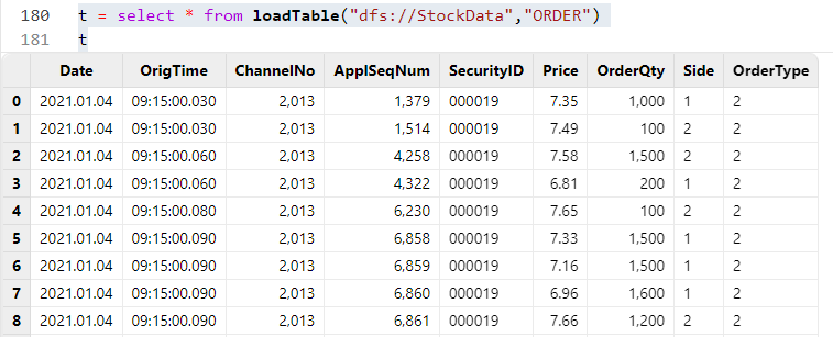
10.2 Solution
t = select * from loadTable("dfs://StockData", "ORDER")By assigning the query result to a variable, you can see the results without issues.
Summary
This tutorial highlights the 10 most commonly overlooked details when programming with DolphinDB, covering various aspects such as partition conflicts, data type handling, metaprogramming, partition pruning, SQL queries, and more. Ignoring these details during programming can lead to errors or unexpected results. By understanding and properly addressing these details, the quality of scripts can be significantly improved, and programming efficiency enhanced.