Best Practices for Array Vectors
Many institutions leverage L1/L2 snapshot market data for quantitative research. DolphinDB, a high-performance real-time computing platform, is optimized for storing and processing large-scale high-frequency market data. To efficiently handle the multi-level structure of snapshot data, DolphinDB implements array vectors that support variable-length two-dimensional arrays. This specialized data strucutre simplifies code for common queries and computations while improving storage and processing performance.
1. Concept
1.1 Overview
In DolphinDB, array vector is a specialized data structure for storing multi-level market data (such as stock bid/ask quotes). Each element of an array vector is a strongly-typed 1D array. This storage method simplifies code for specific queries and computations, while improving data compression and query performance when multiple columns contain redundant data. DolphinDB supports binary operations on array vectors with scalars, vectors, or array vectors, enabling efficient vectorized calculations and boosting performance.
1.2 Array Vector vs. Matrix
Both array vectors and matrices can organize two-dimensional structured data, and their key differences include:
- Matrices require fixed row lengths, whereas array vectors do not.
- Matrices are stored in column-major order, while array vectors use row-major storage.
1.3 Fast Array Vector vs. Columnar Tuple
Array vectors can be further categorized into fast array vectors and columnar tuples. The fast array vector implementation consists of two underlying vectors: one stores all row data contiguously, while the other stores the end indices of each row. This compact storage method delivers efficient read/write and computing performance but makes modifying row lengths challenging. To overcome this limitation, DolphinDB introduced the columnar tuple structure. A columnar tuple represents a column where each element corresponds to a row with consistent value types. Each element in a columnar tuple is an independent object (scalar or vector), allowing for row modifications.
Key Differences
- Fast array vectors currently do not support SYMBOL and STRING types, whereas columnar tuples do.
- When using the
typestrfunction to check data types, fast array vector returns "FAST XXX[] VECTOR", while columnar tuple returns "ANY [<BasicType>]". To check if a variable is a columnar tuple, theisColumnarTuplefunction can be used. - Fast array vector offers higher efficiency in storage, queries, and computations but has lower efficiency in update and delete operations. Additionally, the length of elements in each row cannot be changed. In contrast, columnar tuple performs better in update and delete operations and allows variable row lengths. Note: These update and delete operations are implemented in the underlying C++ code. However, interfaces for updates and deletions are not exposed, meaning script-level modifications or deletions of array vector elements are not supported. Therefore, it is generally recommended for users to use fast array vectors. Unless otherwise specified, "array vectors" generally refers to fast array vectors in DolphinDB documentation.
Application Scenarios
- Fast array vector: Suited for storing and computing numerical two-dimensional arrays, such as 10-level quote data.
- Columnar tuple: Ideal for scenarios that require frequent updates to elements in a two-dimensional array. For instance, reactive state engines automatically convert input fast array vector columns into columnar tuples to enhance the efficiency of state updates. This conversion is transparent to users, who simply need to pass fast array vector columns to the engine.
2. Functions and Operations
2.1 Creation of Array Vectors
2.1.1 Creating Array Vector Variables
Fast Array Vector
Use array or bigarray to define an empty
array vector and populate it with append!:
x = array(INT[], 0).append!([1 2 3, 4 5, 6 7 8, 9 10])
x // output: [[1,2,3],[4,5],[6,7,8],[9,10]]
Use fixedLengthArrayVector to combine
vectors/tuples/matrices/tables into an array vector:
vec = 1 2 3
tp = [4 5 6, 7 8 9]
m = matrix(10 11 12, 13 14 15, 16 17 18)
tb = table(19 20 21 as v1, 22 23 24 as v2)
x = fixedLengthArrayVector(vec, tp, m, tb)
x // output: [[1,4,7,10,13,16,19,22],[2,5,8,11,14,17,20,23],[3,6,9,12,15,18,21,24]]
Use arrayVector to split a single vector into an array
vector:
x = arrayVector(3 5 8 10, [1, 2, 3, 4, 5, 6, 7, 8, 9, 10])
x // output: [[1,2,3],[4,5],[6,7,8],[9,10]]
Columnar Tuple
Use setColumnarTuple! to convert a regular tuple into a
columnar tuple:
x = [[1,2,3],[4,5],[6,7,8],[9,10]].setColumnarTuple!()
x // output: ([1,2,3],[4,5],[6,7,8],[9,10])
2.1.2 Creating Tables With Array Vector Columns
- Assign an array vector as a column in a table:
- Fast array vector columns are typed as "XXX[]" (e.g., "INT[]", "DOUBLE[]").
- Columnar tuple columns are typed as "ANY [<BasicType>] ".
x = array(INT[], 0).append!([1 2 3, 4 5, 6 7 8, 9 10]) y = [1 2 3, 4 5, 6 7 8, 9 10].setColumnarTuple!() t = table(1 2 3 4 as id, x as newCol1) update t set newCol2=x t["newCol3"] = y t /* id newCol1 newCol2 newCol3 -- ------- ------- ------- 1 [1,2,3] [1,2,3] [1,2,3] 2 [4,5] [4,5] [4,5] 3 [6,7,8] [6,7,8] [6,7,8] 4 [9,10] [9,10] [9,10] */ t.schema().colDefs /* name typeString typeInt extra comment ------- ---------- ------- ----- ------- id INT 4 newCol1 INT[] 68 newCol2 INT[] 68 newCol3 ANY[INT] 132 */ - Use
fixedLengthArrayVectorto combine multiple table columns into one array vector column:t = table(1 2 3 4 as id, 1 3 5 6 as v1, 4 7 9 3 as v2) t = select *, fixedLengthArrayVector(v1, v2) as newCol from t t /* id v1 v2 newCol -- -- -- ------ 1 1 4 [1,4] 2 3 7 [3,7] 3 5 9 [5,9] 4 6 3 [6,3] */ - Use
toArrayandgroup byto aggregate grouped data into an array vector:t = table(1 1 3 4 as id, 1 3 5 6 as v1) new_t = select toArray(v1) as newV1 from t group by id new_t /* id newV1 -- ----- 1 [1,3] 3 [5] 4 [6] */Note: Since
toArraygenerates fast array vector data, which does not support SYMBOL or STRING types,toArraycannot be applied to these columns. For grouping SYMBOL or STRING data, use string concatenation instead:t = table(1 1 3 4 as group_id, `a1`a2`a3`a4 as name) new_t = select concat(name, ";") as name from t group by group_id new_t /* group_id name -------- ----- 1 a1;a2 3 a3 4 a4 */Then use
splitin queries to split the concatenated string:select *, name.split(";")[0] as name0 from new_t /* group_id name name0 -------- ----- ----- 1 a1;a2 a1 3 a3 a3 4 a4 a4 */ - Use
loadTextand specify the parameters schema and arrayDelimiter to read tables containing fast array vector columns from text files.When saving withsaveText, fast array vector columns are stored with elements separated by arrayDelimiter:x = array(INT[], 0).append!([1 3 5, 2 7 9]) t = table(1 2 as id, x as value) saveText(t, "./test.csv")Contents of
"./test.csv":id,value 1,"1,3,5" 2,"2,7,9"To load this CSV, specify the column type as "INT[]" in the parameter schema and arrayDelimiter as ",":
t = loadText("./test.csv", schema=table(`id`value as name, ["INT", "INT[]"] as type), arrayDelimiter=",")
t
/*
id value
-- -------
1  [1,3,5]
2  [2,7,9]
*/
2.2 Basic Operations on Array Vectors
2.2.1 Accessing Elements in Array Vectors
Array vector elements can be accessed using functions (row,
at) or positional indexing
(x[index]).
When accessing array vectors using positional indexing,
- If index is a scalar or pair (e.g., 0 or 0:3), it operates on columns.
- If index is a vector (e.g., [1, 2, 3]), it operates on rows.
- Out-of-bounds indices are filled with nulls.
Accessing Rows in Array Vectors
- Use the
rowfunction to retrieve a single row and return a vector.x = array(INT[], 0).append!([1 2 3, 4 5, 6 7 8, 9 10]) x.row(1) // output: [4,5] y = [1 2 3, 4 5, 6 7 8, 9 10].setColumnarTuple!() y.row(1) // output: [4,5] // Out-of-bound: null-filled x.row(10) // output: [,,,] y.row(10) // output: [,,,] - Specify a vector index for positional indexing
x[index]to retrieve rows and return an array vector.x = array(INT[], 0).append!([1 2 3, 4 5, 6 7 8, 9 10]) y = [1 2 3, 4 5, 6 7 8, 9 10].setColumnarTuple!() // Single row x[[1]] // output: [[4,5]] y[[1]] // output: ([4,5]) // Multiple rows x[[1,2]] // output: [[4,5],[6,7,8]] y[[1,2]] // output: ([4,5],[6,7,8]) // Out-of-bound: null-filled x[[3,4]] // output: [[9,10],] y[[3,4]] // output: ([9,10],)
Accessing Columns in Array Vectors
- Specify a scalar index for positional indexing
x[index]to retrieve a single column and return a vector.x = array(INT[], 0).append!([1 2 3, 4 5, 6 7 8, 9 10]) y = [1 2 3, 4 5, 6 7 8, 9 10].setColumnarTuple!() x[1] // output: [2,5,7,10] y[1] // output: [2,5,7,10] // Out-of-bound: null-filled x[10] // output: [,,,] y[10] // output: [,,,] - Specify a pair index for
x[start:end]to retrieve multiple columns and return an array vector.x = array(INT[], 0).append!([1 2 3, 4 5, 6 7 8, 9 10]) y = [1 2 3, 4 5, 6 7 8, 9 10].setColumnarTuple!() // With end specified x[0:2] // output: [[1,2],[4,5],[6,7],[9,10]] y[0:2] // output: [[1,2],[4,5],[6,7],[9,10]] // Open-ended range x[1:] // output: [[2,3],[5],[7,8],[10]] y[1:] // output: ([2,3],[5],[7,8],[10]) // Out-of-bound: null-filled x[1:4] // output: [[2,3,],[5,,],[7,8,],[10,,]] y[1:4] // output: [[2,3,],[5,,],[7,8,],[10,,]]Note:
- start must be ≥0 and < end; otherwise, an exception is thrown.
- For columnar tuple:
- If x is of STRING/SYMBOL type, or end is not specified, the result is a columnar tuple.
- Otherwise, the result is a fast array vector.
Accessing Specific Elements (Row r, Column c)
- Use positional indexing to retrieve elements. For fast array vectors,
use
x[r, c]; For columnar tuples, usex[c, r].x = array(INT[], 0).append!([1 2 3, 4 5, 6 7 8, 9 10]) y = [[1,2,3],[4,5],[6,7,8],[9,10]].setColumnarTuple!() r, c = 2, 1 x[r, c] // output: [7] y[c, r] // output: 7Note:Out-of-bound indices will throw an exception. - Locate elements by row first, and then by
column.
x = array(INT[], 0).append!([1 2 3, 4 5, 6 7 8, 9 10]) y = [[1,2,3],[4,5],[6,7,8],[9,10]].setColumnarTuple!() r, c = 2, 1 rows, cols = [1, 2, 3], 0:2 x.row(r).at(c) // output: 7 y.row(r).at(c) // output: 7 x[[r]][c] // output: [7] y[[r]][c] // output: [7] x[rows][cols] // output: [[4,5],[6,7],[9,10]] y[rows][cols] // output: [[4,5],[6,7],[9,10]] // Out-of-bound: null-filled x[2 3 4][1:3] // output: [[7,8],[10,],[,]] y[2 3 4][1:3] // output: [[7,8],[10,],[,]] - Locate elements by column first, and then by
row.
x = array(INT[], 0).append!([1 2 3, 4 5, 6 7 8, 9 10])
y = [[1,2,3],[4,5],[6,7,8],[9,10]].setColumnarTuple!()
r, c = 2, 1
rows, cols = [1, 2, 3], 0:2

x[c][r]         // output: 7
y[c][r]         // output: 7

x[cols][rows]   // output: [[4,5],[6,7],[9,10]]
y[cols][rows]   // output: [[4,5],[6,7],[9,10]]

x[1:3][2 3 4]   // output: [[7,8],[10,],]
y[1:3][2 3 4]   // output: [[7,8],[10,],]
Accessing Array Vector Columns
To retrieve elements from array vector columns, specify a scalar or pair
index for positional indexing x[index]. Out-of-bound
indices are filled with nulls.
x = array(INT[], 0).append!([1 2 3, 4 5, 6 7 8, 9 10])
y = [1 2 3, 4 5, 6 7 8, 9 10].setColumnarTuple!()
t = table(1 2 3 4 as id, x as x, y as y)
new_t = select *, x[2] as x_newCol1, x[1:3] as x_newCol2, y[2] as y_newCol1, y[1:3] as y_newCol2 from t
new_t

/*
id x       y       x_newCol1 x_newCol2 y_newCol1 y_newCol2
-- ------- ------- --------- --------- --------- ---------
1  [1,2,3] [1,2,3] 3         [2,3]     3         [2,3]
2  [4,5]   [4,5]             [5,]                [5,]
3  [6,7,8] [6,7,8] 8         [7,8]     8         [7,8]
4  [9,10]  [9,10]            [10,]               [10,]
*/
2.2.2 Appending Data to Array Vectors
Currently, array vectors support appending rows, but do not support modifying or deleting elements.
- Use
append!to append rows to array vectors.// Append a single row x = array(INT[], 0).append!([1 2 3, 4 5 6]) x.append!(7) // Append scalar x.append!([8 9]) // Append vector x // output: [[1,2,3],[4,5,6],[7],[8,9]] y = [1 2 3, 4 5 6].setColumnarTuple!() y.append!(7) // Append scalar y.append!([8 9]) // Append vector y // output: ([1,2,3],[4,5,6],7,[8,9]) // Append multiple rows x = array(INT[], 0).append!([1 2 3, 4 5 6]) x.append!([7, 8 9]) x // output: [[1,2,3],[4,5,6],[7],[8,9]] y = [1 2 3, 4 5 6].setColumnarTuple!() y.append!([7, 8 9]) y // output: ([1,2,3],[4,5,6],7,[8,9]) - Use
tableInsertorappend!to add rows to tables containing array vector columns:x = array(INT[], 0).append!([1 2 3, 4 5, 6 7 8, 9 10]) y = [1 2 3, 4 5, 6 7 8, 9 10].setColumnarTuple!() t = table(1 2 3 4 as id, x as col1, y as col2) t.tableInsert(5, 11, 11) t.tableInsert(6, [12 13 14], [12 13 14]) t.append!(table(7 8 as id, [15 16, 17] as col1, [15 16, 17] as col2)) t /* id col1 col2 -- ---------- ---------- 1 [1,2,3] [1,2,3] 2 [4,5] [4,5] 3 [6,7,8] [6,7,8] 4 [9,10] [9,10] 5 [11] 11 6 [12,13,14] [12,13,14] 7 [15,16] [15,16] 8 [17] 17 */
2.2.3 Converting Array Vectors to Vectors and Matrices
- Use the
flattenfunction to convert an array vector into a one-dimensional vector:x = array(INT[], 0).append!([1 2 3, 4 5 6]) z = flatten(x) z // output: [1,2,3,4,5,6] y = [1 2 3, 4 5 6].setColumnarTuple!() z = flatten(y) z // output: [1,2,3,4,5,6] - Use the
matrixfunction to convert equal-length array vectors to matrices:x = array(INT[], 0).append!([1 2 3, 4 5 6]) z = matrix(x) z /* #0 #1 #2 -- -- -- 1 2 3 4 5 6 */ y = [1 2 3, 4 5 6].setColumnarTuple!() z = matrix(y) z /* #0 #1 -- -- 1 4 2 5 3 6 */
2.2.4 Filtering Elements of Fast Array Vectors
Elements of a fast array vector that meet the filtering condition cond
can be filtered out using the syntax x[cond].
x = array(INT[], 0).append!([1 2 3, 4 5, 6 7 8, 9 10])
z = x[x>=5]
z // output: [,[5],[6,7,8],[9,10]]

t = table(1 2 3 4 as id, x as x)
new_t = select *, x[x>=5] as newCol from t
new_t

/*
id x       newCol
-- ------- -------
1  [1,2,3] []
2  [4,5]   [5]
3  [6,7,8] [6,7,8]
4  [9,10]  [9,10]
*/
2.3 Calculations on Array Vectors
2.3.1 Operations With Scalars
The calculation is performed between each element of the array vector and the scalar.
x = array(INT[], 0).append!([1 2 3, 4 5, 6 7 8, 9 10])
z = x + 1
z // output: [[2,3,4],[5,6],[7,8,9],[10,11]]

y = [1 2 3, 4 5, 6 7 8, 9 10].setColumnarTuple!()
z = y + 1
z // output: ([2,3,4],[5,6],[7,8,9],[10,11])

t = table(1 2 3 4 as id, x as x, y as y)
new_t = select *, x + 1 as new_x, y + 1 as new_y from t
new_t

/*
id x       y       new_x   new_y
-- ------- ------- ------- -------
1  [1,2,3] [1,2,3] [2,3,4] [2,3,4]
2  [4,5]   [4,5]   [5,6]   [5,6]
3  [6,7,8] [6,7,8] [7,8,9] [7,8,9]
4  [9,10]  [9,10]  [10,11] [10,11]
*/
2.3.2 Operations With Vectors
The vector length must match the number of rows in the array vector. The calculation is performed between each row of the array vector and the corresponding element in the vector.
x = array(INT[], 0).append!([1 2 3, 4 5, 6 7 8, 9 10])
z = x * [1, 2, 3, 4]
z // output: [[1,2,3],[8,10],[18,21,24],[36,40]]

y = [1 2 3, 4 5, 6 7 8, 9 10].setColumnarTuple!()
z = y * [1, 2, 3, 4]
z // output: ([1,2,3],[8,10],[18,21,24],[36,40])

t = table(1 2 3 4 as id, x as x, y as y)
new_t = select *, x*id as new_x, y*id as new_y from t
new_t

/*
id x       y       new_x      new_y
-- ------- ------- ---------- ----------
1  [1,2,3] [1,2,3] [1,2,3]    [1,2,3]
2  [4,5]   [4,5]   [8,10]     [8,10]
3  [6,7,8] [6,7,8] [18,21,24] [18,21,24]
4  [9,10]  [9,10]  [36,40]    [36,40]
*/
2.3.3 Operations With Array Vectors
The two array vectors must be of the same dimension. The calculation is performed between the corresponding elements of these two array vectors.
x = array(INT[], 0).append!([1 2 3, 4 5, 6 7 8, 9 10])
xx = array(INT[], 0).append!([3 1 2, 3 1, 1 2 3, 0 1])
z = pow(x, xx)
z // output: [[1,2,9],[64,5],[6,49,512],[1,10]]

y = [1 2 3, 4 5, 6 7 8, 9 10].setColumnarTuple!()
yy = [3 1 2, 3 1, 1 2 3, 0 1].setColumnarTuple!()
z = pow(y, yy)
z // output: ([1,2,9],[64,5],[6,49,512],[1,10])

t = table(1 2 3 4 as id, x as x, xx as xx, y as y, yy as yy)
new_t = select *, pow(x, xx) as new_x, pow(y, yy) as new_y from t
new_t

/*
id x       xx      y       yy      new_x      new_y
-- ------- ------- ------- ------- ---------- ----------
1  [1,2,3] [3,1,2] [1,2,3] [3,1,2] [1,2,9]    [1,2,9]
2  [4,5]   [3,1]   [4,5]   [3,1]   [64,5]     [64,5]
3  [6,7,8] [1,2,3] [6,7,8] [1,2,3] [6,49,512] [6,49,512]
4  [9,10]  [0,1]   [9,10]  [0,1]   [1,10]     [1,10]
*/
Note that direct calculations between fast array vectors and columnar tuples are not supported.
2.3.4 Row-Based Calculations
Row-Based Functions
Row-based functions
support array vectors. These functions are named in the format
rowFunc, such as rowSum,
rowAlign, etc.
- Unary functions: row-wise
sum
x = array(INT[], 0).append!([1 2 3, 4 5, 6 7 8, 9 10]) z = rowSum(x) z // output: [6,9,21,19] y = [1 2 3, 4 5, 6 7 8, 9 10].setColumnarTuple!() z = rowSum(y) z // output: [6,9,21,19] t = table(1 2 3 4 as id, x as x, y as y) new_t = select *, rowSum(x) as new_x, rowSum(y) as new_y from t new_t /* id x y new_x new_y -- ------- ------- ----- ----- 1 [1,2,3] [1,2,3] 6 6 2 [4,5] [4,5] 9 9 3 [6,7,8] [6,7,8] 21 21 4 [9,10] [9,10] 19 19 */ - Binary operations (on array vectors and vectors): Row-wise weighted
average
x = array(INT[], 0).append!([1 2 3, 4 5 6, 6 7 8, 9 10 11]) z = rowWavg(x, [1, 1, 2]) z // output: [2.25,5.25,7.25,10.25] y = [1 2 3, 4 5 6, 6 7 8, 9 10 11].setColumnarTuple!() z = rowWavg(y, [1, 1, 2]) z // output: [2.25,5.25,7.25,10.25] t = table(1 2 3 4 as id, x as x, y as y) new_t = select *, rowWavg(x, [1, 1, 2]) as new_x, rowWavg(y, [1, 1, 2]) as new_y from t new_t /* id x y new_x new_y -- --------- --------- ----- ----- 1 [1,2,3] [1,2,3] 2.25 2.25 2 [4,5,6] [4,5,6] 5.25 5.25 3 [6,7,8] [6,7,8] 7.25 7.25 4 [9,10,11] [9,10,11] 10.25 10.25 */ - Binary operations (on array vectors and array vectors): Row-wise
correlation
coefficient
x = array(INT[], 0).append!([1 2 3, 4 5, 6 7 8, 9 10]) xx = array(INT[], 0).append!([3 1 2, 3 1, 1 2 3, 0 1]) z = rowCorr(x, xx) z // output: [-0.5,-1,1,1] y = [1 2 3, 4 5, 6 7 8, 9 10].setColumnarTuple!() yy = [3 1 2, 3 1, 1 2 3, 0 1].setColumnarTuple!() z = rowCorr(y, yy) z // output: [-0.5,-1,1,1] t = table(1 2 3 4 as id, x as x, xx as xx, y as y, yy as yy) new_t = select *, rowCorr(x, xx) as new_x, rowCorr(y, yy) as new_y from t new_t /* id x xx y yy new_x new_y -- ------- ------- ------- ------- ----- ----- 1 [1,2,3] [3,1,2] [1,2,3] [3,1,2] -0.5 -0.5 2 [4,5] [3,1] [4,5] [3,1] -1 -1 3 [6,7,8] [1,2,3] [6,7,8] [1,2,3] 1 1 4 [9,10] [0,1] [9,10] [0,1] 1 1 */ - Special Binary Operations: row-wise alignment
For special data alignment rules in financial scenarios, DolphinDB provides the rowAlign and rowAt functions:
rowAlign(left, right, how)aligns the left and right array vectors based on specified alignment rules.rowAt(X, [Y])retrieves the row indices for each true element in X.left = array(DOUBLE[], 0).append!([9.00 8.98 8.97 8.96 8.95, 8.99 8.97 8.95 8.93 8.91]) right = prev(left) left // output: [[9,8.98,8.97,8.96,8.949999999999999],[8.99,8.97,8.949999999999999,8.929999999999999,8.91]] right // output: [,[9,8.98,8.97,8.96,8.949999999999999]] leftIndex, rightIndex = rowAlign(left, right, how="bid") leftIndex // output: [[0,1,2,3,4],[-1,0,-1,1,-1,2]] rightIndex // output: [[-1,-1,-1,-1,-1],[0,-1,1,2,3,4]] leftResult = rowAt(left, leftIndex) rightResult = rowAt(right, rightIndex) leftResult // output: [[9,8.98,8.97,8.96,8.949999999999999],[,8.99,,8.97,,8.949999999999999]] rightResult // output: [[,,,,],[9,,8.98,8.97,8.96,8.949999999999999]]
Higher-Order Function byRow
The higher-order function byRow can be called on fast array
vectors to apply a user-defined function on each row element.
For example, calculate cumulative sum for each row:
x = array(INT[], 0).append!([1 2 3, 4 5, 6 7 8, 9 10])
z = byRow(cumsum, x)
z // output: [[1,3,6],[4,9],[6,13,21],[9,19]]

t = table(1 2 3 4 as id, x as x)
new_t = select *, byRow(cumsum, x) as new_x from t
new_t

/*
id x       new_x
-- ------- ---------
1  [1,2,3] [1,3,6]
2  [4,5]   [4,9]
3  [6,7,8] [6,13,21]
4  [9,10]  [9,19]
*/Note:
byRowonly supports fast array vectors.- When using the
byRowfunction, the return value of func can only be a scalar or a vector of the same length as the array vector.
// Return value is a scalar
defg foo1(v){
    return last(v)-first(v)
}

// Return value is a vector of the same length as v
def foo2(v){
    return v \ prev(v) - 1
}

x = array(INT[], 0).append!([1 2 3, 4 5, 6 7 8, 9 10])
x1 = byRow(foo1, x)
x2 = byRow(foo2, x)

x1 // output: [2,1,2,1]
x2 // output: [[,1,0.5],[,0.25],[,0.166666666666667,0.142857142857143],[,0.111111111111111]]

t = table(1 2 3 4 as id, x as x)
new_t = select *, byRow(foo1, x) as x1, byRow(foo2, x) as x2 from t
new_t

/*
id x       x1 x2
-- ------- -- --------------------------------------
1  [1,2,3] 2  [,1,0.5]
2  [4,5]   1  [,0.25]
3  [6,7,8] 2  [,0.166666666666667,0.142857142857143]
4  [9,10]  1  [,0.111111111111111]
*/
Higher-Order Functions each and
loop
The higher-order functions each and loop
can be called on array vectors to apply a user-defined function on each row
element. Their differences are:
byRowonly supports fast array vectors, whileeachandloopsupport both fast array vectors and columnar tuples.- For
eachandloop, there is no limitation on the return value of func, and it can be a vector of different lengths from the input row elements. If the return value of func is a vector, the result is a tuple, and the corresponding column in the table is columnar tuple. - For
byRow, if the return value of func is a vector, the result ofbyRowis a fast array vector, and the corresponding column in the table is a fast array vector.
// Return value can be a vector of different length from v
def foo3(v){
    return [last(v)-first(v), last(v)+first(v)]
}

x = array(INT[], 0).append!([1 2 3, 4 5, 6 7 8, 9 10])
z = loop(foo3, x)
z // output: ([2,4],[1,9],[2,14],[1,19])

y = [1 2 3, 4 5, 6 7 8, 9 10].setColumnarTuple!()
z = loop(foo3, y)
z // output: ([2,4],[1,9],[2,14],[1,19])

t = table(1 2 3 4 as id, x as x, y as y)
new_t = select *, loop(foo3, x) as new_x, loop(foo3, y) as new_y from t
new_t

/*
id x       y       new_x  new_y
-- ------- ------- ------ ------
1  [1,2,3] [1,2,3] [2,4]  [2,4]
2  [4,5]   [4,5]   [1,9]  [1,9]
3  [6,7,8] [6,7,8] [2,14] [2,14]
4  [9,10]  [9,10]  [1,19] [1,19]
*/
2.4 API Writing
2.4.1 C++ API
int rowNum = 3;   // Row number
int elementsPerRow = 3;    // Number of elements per row
vector<string> colNames = {"id", "value"};
vector<DATA_TYPE> colTypes = {DT_INT, DT_DOUBLE_ARRAY};createArrayVector.// Create an index vector
VectorSP indexVector = Util::createVector(DT_INDEX, rowNum, rowNum);
INDEX* pindex = indexVector->getIndexArray();
int cumulative = 0;
for (int i = 0; i < rowNum; ++i) {
cumulative += elementsPerRow;
pindex[i] = cumulative;
}
// Create a value vector
VectorSP valueVector = Util::createVector(DT_DOUBLE, rowNum * elementsPerRow, rowNum * elementsPerRow);
int valueIndex = 0;
for (int i = 0; i < rowNum; ++i) {
for (int j = 0; j < elementsPerRow; ++j) {
valueVector->setDouble(valueIndex++, i * 3 + j + 0.1);
}
}
// Create an array vector
VectorSP arrayVectorCol = Util::createArrayVector(indexVector, valueVector);// Create the id column
VectorSP idCol = Util::createVector(DT_INT, rowNum, rowNum);
for (int i = 0; i < rowNum; ++i) {
idCol->setInt(i, i);
}
// Create the table
vector<ConstantSP> cols = {idCol, arrayVectorCol};
ConstantSP table = Util::createTable(colNames, cols);upload method. For details, see User Manual > C++
API.// Connect to DolphinDB
DBConnection conn;
bool connected = conn.connect("127.0.0.1", 8848);
if (!connected) {
cout << "Failed to connect to DolphinDB server" << endl;
return -1;
}
// Log in to DolphinDB
conn.login("admin", "123456", false);
cout << "Login successful" << endl;
// Upload data
conn.upload("myArrayVectorTable", table);
cout << "Table uploaded using createArrayVector successfully" << endl;
// Query data
string script = "select * from myArrayVectorTable;";
ConstantSP result = conn.run(script);
cout << "------ Data Verification ------" << endl;
cout << result->getString() << endl;
conn.close();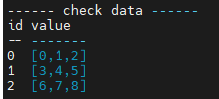
2.4.2 Java API
Connect & Create Table
Connect to DolphinDB and create a dimension table to receive data. Specify the column type as XX[]. For example, in the following case, the value column is an INT array vector, so it is specified as INT[].
// Connect to the DolphinDB
DBConnection conn = new DBConnection();
boolean success = conn.connect("127.0.0.1", 8848, "admin", "123456");
// Create a dimension table
String ddb_script = "dbName = \"dfs://testDB\"\n" +"../py_api.dita"est\"\n" +
                "if(existsDatabase(dbName)) {\n" +
                "    dropDatabase(dbName)\n" +
                "}\n" +
                "db = database(dbName, VALUE, 1 2 3 4, , 'TSDB')\n" +
                "schemaTB = table(1:0, `id`value, [INT, INT[]])\n" +
                "pt = createTable(db, schemaTB, tbName, sortColumns=`id)";
conn.run(ddb_script);
Construct Data
Construct data in Java and create a table object. Each column corresponds to a list, and the array vector column is a list of type vector, where each row is a vector.
List<String> colNames = Arrays.asList("id", "value");
List<Vector> cols = new ArrayList<>(6);
int rowNum = 4;
List<Integer> idCol = new ArrayList<>(rowNum);
List<Vector> valueCol = new ArrayList<>(rowNum);    // array vector column
for(int i = 0; i < rowNum; ++i) {
    idCol.add(i + 1);
    List<Integer> valueRow = new ArrayList<>(50);   // A row in the array vector
    for(int j = 0; j < 3; ++j) {
        valueRow.add(i*3 +j);
    }
    valueCol.add(new BasicIntVector(valueRow));
}
cols.add(new BasicIntVector(idCol));
cols.add(new BasicArrayVector(valueCol));
BasicTable tb = new BasicTable(colNames, cols);
Upload Data
Insert data into the dimension table. In the example, the table data tb is
uploaded to the dimension table (loaded by
loadTable('dfs://testDB','test')) using the
tableInsert method. For details, see User Manual > Java API.
List<Entity> tbArg = new ArrayList<>(1);
tbArg.add(tb);
conn.run("tableInsert{loadTable('dfs://testDB','test')}", tbArg);
Query Data
BasicTable t;
t = (BasicTable)conn.run("select * from loadTable('dfs://testDB','test')");
System.out.println(t.getString());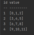
2.4.3 Python API
Construct Data
Create a table object in Python. For example, in the following case, the value column is an INT array vector.
df = pd.DataFrame({
    'id': [1, 2, 3, 4],
    'value': [np.array([1,2,3],dtype=np.int64), np.array([4,5,6],dtype=np.int64), np.array([7,8,9],dtype=np.int64), np.array([10,11,12],dtype=np.int64)]
})
Upload Data
Connect to DolphinDB and upload the data. In the example, the DataFrame df is
uploaded to the in-memory table myTable in DolphinDB using the
table method. For details, see User Manual > Python API.
# Connect to the DolphinDB
s = ddb.session()
s.connect("127.0.0.1", 8848, "admin", "123456")
# Upload data to the in-memory table
s.table(data=df, tableAliasName="myTable")
Query Data
t = s.run("select * from myTable")
print(t)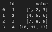
3. Application in Level 2 Snapshot Data
3.1 Storing Snapshot Data
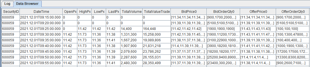
A typical application scenario for array vector is storing Level 2 snapshot data. The Level 2 data usually contains 10-level bid/ask prices, trade volumes, trade counts, first 50 bid/ask orders, and other multi-level data. Level 2 snapshot data often needs to be processed by dataset, so it is optimal to store multi-level market data using array vector columns.


The following table shows the table schema used in this tutorial:
| Field Name | Data Type |
|---|---|
| SecurityID | SYMBOL |
| DateTime | TIMESTAMP |
| PreClosePx | DOUBLE |
| OpenPx | DOUBLE |
| HighPx | DOUBLE |
| LowPx | DOUBLE |
| LastPx | DOUBLE |
| TotalVolumeTrade | INT |
| TotalValueTrade | DOUBLE |
| InstrumentStatus | SYMBOL |
| BidPrice | DOUBLE[] |
| BidOrderQty | INT[] |
| BidNumOrders | INT[] |
| BidOrders | INT[] |
| OfferPrice | DOUBLE[] |
| OfferOrderQty | INT[] |
| OfferNumOrders | INT[] |
| OfferOrders | INT[] |
| NumTrades | INT |
| IOPV | DOUBLE |
| TotalBidQty | INT |
| TotalOfferQty | INT |
| WeightedAvgBidPx | DOUBLE |
| WeightedAvgOfferPx | DOUBLE |
| TotalBidNumber | INT |
| TotalOfferNumber | INT |
| BidTradeMaxDuration | INT |
| OfferTradeMaxDuration | INT |
| NumBidOrders | INT |
| NumOfferOrders | INT |
| WithdrawBuyNumber | INT |
| WithdrawBuyAmount | INT |
| WithdrawBuyMoney | DOUBLE |
| WithdrawSellNumber | INT |
| WithdrawSellAmount | INT |
| WithdrawSellMoney | DOUBLE |
| ETFBuyNumber | INT |
| ETFBuyAmount | INT |
| ETFBuyMoney | DOUBLE |
| ETFSellNumber | INT |
| ETFSellAmount | INT |
| ETFSellMoney | DOUBLE |
Eight fields (BidPrice, OfferPrice, BidOrderQty, OfferOrderQty, BidNumOrders, OfferNumOrders, BidOrders, OfferOrders) use the array vector structure. Column types are specified as DOUBLE[] and INT[] during table creation. Use the following script to create the table:
dbName = "dfs://SH_TSDB_snapshot_ArrayVector"
tbName = "snapshot"
if(existsDatabase(dbName)){
 dropDatabase(dbName)
}
db1 = database(, VALUE, 2020.01.01..2021.01.01)
db2 = database(, HASH, [SYMBOL, 20])
db = database(dbName, COMPO, [db1, db2], , "TSDB")
schemaTable = table(
 array(SYMBOL, 0) as SecurityID,
 array(TIMESTAMP, 0) as DateTime,
 array(DOUBLE, 0) as PreClosePx,
 array(DOUBLE, 0) as OpenPx,
 array(DOUBLE, 0) as HighPx,
 array(DOUBLE, 0) as LowPx,
 array(DOUBLE, 0) as LastPx,
 array(INT, 0) as TotalVolumeTrade,
 array(DOUBLE, 0) as TotalValueTrade,
 array(SYMBOL, 0) as InstrumentStatus,
 array(DOUBLE[], 0) as BidPrice,
 array(INT[], 0) as BidOrderQty,
 array(INT[], 0) as BidNumOrders,
 array(INT[], 0) as BidOrders,
 array(DOUBLE[], 0) as OfferPrice,
 array(INT[], 0) as OfferOrderQty,
 array(INT[], 0) as OfferNumOrders,
 array(INT[], 0) as OfferOrders,
 array(INT, 0) as NumTrades,
 array(DOUBLE, 0) as IOPV,
 array(INT, 0) as TotalBidQty,
 array(INT, 0) as TotalOfferQty,
 array(DOUBLE, 0) as WeightedAvgBidPx,
 array(DOUBLE, 0) as WeightedAvgOfferPx,
 array(INT, 0) as TotalBidNumber,
 array(INT, 0) as TotalOfferNumber,
 array(INT, 0) as BidTradeMaxDuration,
 array(INT, 0) as OfferTradeMaxDuration,
 array(INT, 0) as NumBidOrders,
 array(INT, 0) as NumOfferOrders,
 array(INT, 0) as WithdrawBuyNumber,
 array(INT, 0) as WithdrawBuyAmount,
 array(DOUBLE, 0) as WithdrawBuyMoney,
 array(INT, 0) as WithdrawSellNumber,
 array(INT, 0) as WithdrawSellAmount,
 array(DOUBLE, 0) as WithdrawSellMoney,
 array(INT, 0) as ETFBuyNumber,
 array(INT, 0) as ETFBuyAmount,
 array(DOUBLE, 0) as ETFBuyMoney,
 array(INT, 0) as ETFSellNumber,
 array(INT, 0) as ETFSellAmount,
 array(DOUBLE, 0) as ETFSellMoney
)
db.createPartitionedTable(table=schemaTable, tableName=tbName, partitionColumns=`DateTime`SecurityID, compressMethods={DateTime:"delta"}, sortColumns=`SecurityID`DateTime, keepDuplicates=ALL)
During data import, the fixedLengthArrayVector function combines
multi-level data into single array vector columns. The data import script:
 def transform(data){
 t = select SecurityID, DateTime, PreClosePx, OpenPx, HighPx, LowPx, LastPx, TotalVolumeTrade, TotalValueTrade, InstrumentStatus,
        fixedLengthArrayVector(BidPrice0, BidPrice1, BidPrice2, BidPrice3,  BidPrice4, BidPrice5, BidPrice6, BidPrice7, BidPrice8, BidPrice9) as BidPrice,
        fixedLengthArrayVector(BidOrderQty0, BidOrderQty1, BidOrderQty2, BidOrderQty3,  BidOrderQty4, BidOrderQty5, BidOrderQty6, BidOrderQty7, BidOrderQty8, BidOrderQty9) as BidOrderQty,
        fixedLengthArrayVector(BidNumOrders0, BidNumOrders1, BidNumOrders2, BidNumOrders3,  BidNumOrders4, BidNumOrders5, BidNumOrders6, BidNumOrders7, BidNumOrders8, BidNumOrders9) as BidNumOrders,
        fixedLengthArrayVector(BidOrders0, BidOrders1, BidOrders2, BidOrders3,  BidOrders4, BidOrders5, BidOrders6, BidOrders7, BidOrders8, BidOrders9, BidOrders10, BidOrders11, BidOrders12, BidOrders13,  BidOrders14, BidOrders15, BidOrders16, BidOrders17, BidOrders18, BidOrders19, BidOrders20, BidOrders21, BidOrders22, BidOrders23,  BidOrders24, BidOrders25, BidOrders26, BidOrders27, BidOrders28, BidOrders29, BidOrders30, BidOrders31, BidOrders32, BidOrders33,  BidOrders34, BidOrders35, BidOrders36, BidOrders37, BidOrders38, BidOrders39, BidOrders40, BidOrders41, BidOrders42, BidOrders43,  BidOrders44, BidOrders45, BidOrders46, BidOrders47, BidOrders48, BidOrders49) as BidOrders,
        fixedLengthArrayVector(OfferPrice0, OfferPrice1, OfferPrice2, OfferPrice3,  OfferPrice4, OfferPrice5, OfferPrice6, OfferPrice7, OfferPrice8, OfferPrice9) as OfferPrice,
        fixedLengthArrayVector(OfferOrderQty0, OfferOrderQty1, OfferOrderQty2, OfferOrderQty3,  OfferOrderQty4, OfferOrderQty5, OfferOrderQty6, OfferOrderQty7, OfferOrderQty8, OfferOrderQty9) as OfferOrderQty,
        fixedLengthArrayVector(OfferNumOrders0, OfferNumOrders1, OfferNumOrders2, OfferNumOrders3,  OfferNumOrders4, OfferNumOrders5, OfferNumOrders6, OfferNumOrders7, OfferNumOrders8, OfferNumOrders9) as OfferNumOrders,
        fixedLengthArrayVector(OfferOrders0, OfferOrders1, OfferOrders2, OfferOrders3,  OfferOrders4, OfferOrders5, OfferOrders6, OfferOrders7, OfferOrders8, OfferOrders9, OfferOrders10, OfferOrders11, OfferOrders12, OfferOrders13,  OfferOrders14, OfferOrders15, OfferOrders16, OfferOrders17, OfferOrders18, OfferOrders19, OfferOrders20, OfferOrders21, OfferOrders22, OfferOrders23,  OfferOrders24, OfferOrders25, OfferOrders26, OfferOrders27, OfferOrders28, OfferOrders29, OfferOrders30, OfferOrders31, OfferOrders32, OfferOrders33,  OfferOrders34, OfferOrders35, OfferOrders36, OfferOrders37, OfferOrders38, OfferOrders39, OfferOrders40, OfferOrders41, OfferOrders42, OfferOrders43,  OfferOrders44, OfferOrders45, OfferOrders46, OfferOrders47, OfferOrders48, OfferOrders49) as OfferOrders,
        NumTrades, IOPV, TotalBidQty, TotalOfferQty, WeightedAvgBidPx, WeightedAvgOfferPx, TotalBidNumber, TotalOfferNumber, BidTradeMaxDuration,OfferTradeMaxDuration, NumBidOrders, NumOfferOrders, WithdrawBuyNumber, WithdrawBuyAmount, WithdrawBuyMoney,WithdrawSellNumber, WithdrawSellAmount, WithdrawSellMoney, ETFBuyNumber, ETFBuyAmount, ETFBuyMoney, ETFSellNumber, ETFSellAmount, ETFSellMoney
        from data
 return t
}

def loadData(csvDir, dbName, tbName){
 schemaTB = extractTextSchema(csvDir)
 update schemaTB set type = "SYMBOL" where name = "SecurityID"
 loadTextEx(dbHandle=database(dbName), tableName=tbName, partitionColumns=`DateTime`SecurityID, sortColumns=`SecurityID`DateTime, filename=csvDir, schema=schemaTB, transform=transform)
}

// Submit import job
csvDir = "/home/v2/data/testdata/snapshot_100stocks_multi.csv"
dbName, tbName = "dfs://SH_TSDB_snapshot_ArrayVector", "snapshot"
submitJob("loadData", "load Data", loadData{csvDir, dbName, tbName})
getRecentJobs()
3.2 Storing Raw Data in Grouped Calculation
Another key application of array vectors is storing original data during grouped
aggregations. DolphinDB provides the toArray function, which
can be combined with group by to store data in each group as a
row in an array vector column, enabling users to directly examine all data
within each group.
For example, aggregating snapshot data by 5 minute while preserving bid/ask prices and volumes:
// Create database for 5-minute bars
def createFiveMinuteBarDB(dbName, tbName){
 if(existsDatabase(dbName)){
  dropDatabase(dbName)
 }
 db = database(dbName, VALUE, 2021.01.01..2021.12.31, , "TSDB")
 colNames = `SecurityID`DateTime`OpenPx`HighPx`LowPx`LastPx`TotalVolume`TotalValueTrade`BidPrice0`BidOrderQty0`OfferPrice0`OfferOrderQty0
 colTypes = [SYMBOL, TIMESTAMP, DOUBLE, DOUBLE, DOUBLE, DOUBLE, LONG, DOUBLE, DOUBLE[], INT[], DOUBLE[], INT[]]
 schemaTable = table(1:0, colNames, colTypes)
 db.createPartitionedTable(table=schemaTable, tableName=tbName, partitionColumns=`DateTime, compressMethods={DateTime:"delta"}, sortColumns=`SecurityID`DateTime, keepDuplicates=ALL)
}
dbName, tbName = "dfs://fiveMinuteBar", "fiveMinuteBar"
createFiveMinuteBarDB(dbName, tbName)

// Calculate 5-minute bars from snapshot data
t = select first(OpenPx) as OpenPx, max(HighPx) as HighPx, min(LowPx) as LowPx, last(LastPx) as LastPx, last(TotalVolumeTrade) as TotalVolumeTrade, last(TotalValueTrade) as TotalValueTrade, toArray(BidPrice[0]) as BidPrice0,  toArray(BidOrderQty[0]) as BidOrderQty0, toArray(OfferPrice[0]) as OfferPrice0, toArray(OfferOrderQty[0]) as OfferOrderQty0 from loadTable("dfs://SH_TSDB_snapshot_ArrayVector", "snapshot") group by SecurityID, interval(DateTime, 5m, "none") as DateTime map

// Save results
loadTable(dbName, tbName).append!(t)
3.3 High-Frequency Factor Calculation Using Snapshot Data
DolphinDB not only provides high-performance access to time series data but also features a built-in vectorized programming language and powerful computing engines, making it efficient for quantitative finance factor development. This includes high-frequency factor calculation based on historical data and stream computation based on real-time Level 2 market data. This section demonstrates the application of array vectors in factor calculation, using high-frequency factor computation based on snapshot data as an example.
3.3.1 Net Incremental Buying Amount
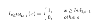
The formula for calculating net incremental buying amount is defined as follows:
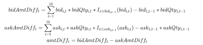
Where bidAmtDifft represents the buying order increment at time t; bidi,t represents the i-th level bid price at time t in the snapshot data; the indicator function I is defined as:
The following script implements the factor based on the formula and DolphinDB built-in functions:
@state
def calculateAmtDiff(bid, ask, bidvol, askvol){
    lastBidPrice = prev(bid[0])  // Best bid price of the previous tick
    lastAskPrice = prev(ask[0])  // Best ask price of the previous tick
    lastBidQty = prev(bidvol[0])  // Best bid quantity of the previous tick
    lastAskQty = prev(askvol[0])  // Best ask quantity of the previous tick
    // Calculate buying order increment
    bidAmtDiff = rowSum(bid*bidvol*(bid >= lastBidPrice)) - lastBidPrice*lastBidQty
    // Calculate selling order increment
    askAmtDiff = rowSum(ask*askvol*(ask <= lastAskPrice)) - lastAskPrice*lastAsk
    return bidAmtDiff - askAmtDiff
}
The prev function is used to retrieve the price of the the
previous tick, and the rowSum function calculates the sum
by row of the array vector column.
Batch Processing
snapshot = loadTable("dfs://SH_TSDB_snapshot_ArrayVector", "snapshot")
res1 = select SecurityID, DateTime, calculateAmtDiff(BidPrice, OfferPrice, BidOrderQty, OfferOrderQty) as amtDiff from snapshot context by SecurityID csort DateTime
Stream Processing
// Create input and output tables
share(streamTable(1:0, snapshot.schema().colDefs.name, snapshot.schema().colDefs.typeString), `snapshotStreamTable)
share(streamTable(1:0, `SecurityID`DateTime`amtDiff, [SYMBOL, TIMESTAMP, DOUBLE]), `res2)
go
// Create streaming engine
createReactiveStateEngine(name="calAmtDiffDemo", metrics=<[DateTime, calculateAmtDiff(BidPrice, OfferPrice, BidOrderQty, OfferOrderQty)]>, dummyTable=snapshotStreamTable, outputTable=res2, keyColumn=`SecurityID)
// Subscribe to snapshot data
subscribeTable(tableName="snapshotStreamTable", actionName="calAmtDiffTest", offset=-1, handler=getStreamEngine("calAmtDiffDemo"), msgAsTable=true)
// Replay data to simulate streams
testData = select * from snapshot where date(DateTime)=2021.12.01 order by DateTime
submitJob("replayData", "replay snapshot data", replay{inputTables=testData, outputTables=snapshotStreamTable, dateColumn=`DateTime, timeColumn=`DateTime, replayRate=1000})
3.3.2 10-Level Net Incremental Buying Amount
The formula for calculating 10-level net incremental buying amount is defined as follows:
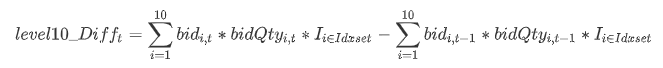
Where level10_Difft represents the buying order increment at time t; bidi,t represents the i-th level bid price at time t in the snapshot data; the indicator function I is defined as:
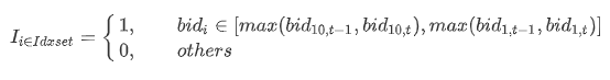
The following script implements the factor using DolphinDB built-in functions:
@state
def level10_Diff(price, qty, buy){
        prevPrice = price.prev()
        left, right = rowAlign(price, prevPrice, how=iif(buy, "bid", "ask"))
        qtyDiff = (qty.rowAt(left).nullFill(0) - qty.prev().rowAt(right).nullFill(0))
        amtDiff = rowSum(nullFill(price.rowAt(left), prevPrice.rowAt(right)) * qtyDiff)
        return amtDiff
}

snapshot = loadTable("dfs://SH_TSDB_snapshot_ArrayVector", "snapshot")
res = select SecurityID, DateTime, level10_Diff(BidPrice, BidOrderQty, true) as level10_Diff from snapshot context by SecurityID csort DateTime
The row alignment function rowAlign is used to align the
current and previous 10-level prices. The rowAt and
nullFill functions are used to retrieve the
corresponding level's order volume and price. Finally, the total change
amount is calculated using the rowSum function.
4. Conclusion
This tutorial introduced DolphinDB's array vector structure for efficient variable-length 2D array storage and computation, detailing its key features, usage, and applications. DolphinDB’s capability for storing and processing large-scale high-frequency market data makes it an ideal solution for factor development. Array vectors offer a simple, efficient, and flexible approach, particularly suited for handling Level 2 snapshot data.