
Calculate Daily Cumulative Order-by-Order Capital Flow in Real Time
In the stock market, capital flow is an important price-volume indicator. Capital flow indicators can be classified by whether trade order IDs are consolidated: tick-by-tick capital flow and order-by-order capital flow. They can also be classified by the aggregation period: minute-level capital flow and daily cumulative capital flow. The processing logic for tick-by-tick capital flow is relatively straightforward. Each trade record is classified by order size based on its trading volume or trading value, and the relevant indicators are then calculated. Order-by-order capital flow is more complex. Trades must first be consolidated by buy and sell order IDs before order-size classification and indicator calculation can be performed.
For a solution that calculates minute-level order-by-order capital flow in real time, see the tutorial: Calculate Minute-Level Capital Flow in Real Time.
This tutorial provides a low-latency solution for calculating daily cumulative order-by-order capital flow in real time based on the DolphinDB streaming processing framework.
Note: In subsequent sections, “daily cumulative capital flow” refers to daily cumulative order-by-order capital flow.
1. Daily Cumulative Capital Flow Scenario
1.1. Challenges in Calculating Daily Cumulative Capital Flow in Real Time
-
In daily cumulative capital flow calculations, order size is dynamic: a small order may become a large order after its trading volume increases.
-
The calculation depends on the historical state. Without incremental calculation, processing afternoon data may require checking the morning data for the same order, which is highly inefficient.
-
This scenario requires processing every trade record and calculating the latest daily cumulative capital flow indicators for each stock up to the current trade record, posing a challenge for real-time computation.
-
The calculation involves at least two stages. In the first stage, trades are grouped by order, and the cumulative trading volume of each order is used to classify its size. In the second stage, data is grouped by stock to calculate the number of orders and trading value for each order-size category.
-
Low latency is required in real-time stream processing scenarios.
1.2. Tick-by-Tick Trade Data
This tutorial uses tick-by-tick trade data from a trading day in 2020 on the Shanghai Stock Exchange for code debugging. The table schema stored in DolphinDB is as follows (returned by schema(t).colDefs):
| name | typeString | comment |
|---|---|---|
| SecurityID | SYMBOL | Stock code |
| Market | SYMBOL | Exchange |
| TradeTime | TIMESTAMP | Trade time |
| TradePrice | DOUBLE | Trade price |
| TradeQty | INT | Trading volume |
| TradeAmount | DOUBLE | Trading value |
| BuyNum | INT | Buy order ID |
| SellNum | INT | Sell order ID |
1.3. Daily Cumulative Capital Flow Indicators
The sample code in this tutorial calculates the following daily cumulative capital flow indicators:
| Metric Name | Description |
|---|---|
| TotalAmount | Total trading value from market open to the current tick |
| SellSmallAmount | Total trading value of small sell-side orders from market open to the current tick, where trading volume is less than or equal to 20,000 shares |
| SellMediumAmount | Total trading value of medium sell-side orders from market open to the current tick, where trading volume is greater than 20,000 shares and less than or equal to 200,000 shares |
| SellBigAmount | Total trading value of large sell-side orders from market open to the current tick, where trading volume is greater than 200,000 shares |
| SellSmallCount | Total number of small sell-side orders from market open to the current tick, where trading volume is less than or equal to 20,000 shares |
| SellMediumCount | Total number of medium sell-side orders from market open to the current tick, where trading volume is greater than 20,000 shares and less than or equal to 200,000 shares |
| SellBigCount | Total number of large sell-side orders from market open to the current tick, where trading volume is greater than 200,000 shares |
| BuySmallAmount | Total trading value of small buy-side orders from market open to the current tick, where trading volume is less than or equal to 20,000 shares |
| BuyMediumAmount | Total trading value of medium buy-side orders from market open to the current tick, where trading volume is greater than 20,000 shares and less than or equal to 200,000 shares |
| BuyBigAmount | Total trading value of large buy-side orders from market open to the current tick, where trading volume is greater than 200,000 shares |
| BuySmallCount | Total number of small buy-side orders from market open to the current tick, where trading volume is less than or equal to 20,000 shares |
| BuyMediumCount | Total number of medium buy-side orders from market open to the current tick, where trading volume is greater than 20,000 shares and less than or equal to 200,000 shares |
| BuyBigCount | Total number of large buy-side orders from market open to the current tick, where trading volume is greater than 200,000 shares |
There is no universal rule for classifying large and small orders in capital flow analysis. Different criteria can be used depending on the application. For example, common stock market data applications use the following rules:
(1) Eastmoney
-
Extra-large order: >500,000 shares or CNY 1,000,000
-
Large order: 100,000-500,000 shares or CNY 200,000-1,000,000
-
Medium order: 20,000-100,000 shares or CNY 40,000-200,000
-
Small order: <20,000 shares or CNY 40,000
(2) Sina Finance
-
Extra-large order: >CNY 1,000,000
-
Large order: CNY 200,000-1,000,000
-
Small order: CNY 50,000-200,000
-
Very small order: <CNY 50,000
Different applications also use different rules to distinguish order sizes, but their criteria are all based on trading volume or trading value.
Note: In this tutorial, capital flow order-size classification is based on trading volume and uses three categories: large, medium, and small orders. The threshold values are defined arbitrarily, and you must adjust them for your own scenario.
1.4. Incremental Calculation Solution for Daily Cumulative Capital Flow
Incremental calculation of daily cumulative order-by-order capital flow consists of two steps. First, calculate the cumulative trading volume for each buy or sell order, and use it to classify the order as large, medium, or small. This step is relatively simple to implement incrementally: group by order and use cumsum to calculate cumulative trading volume. Then, aggregate by stock to calculate indicators such as the number of orders and trading value for each order-size category. Without incremental calculation in this step, each aggregation of large, medium, and small order counts takes longer over time because the number of orders keeps increasing. In fact, if we can obtain both the current state of an order (large, medium, small, and so on) and its previous state, the incremental calculation in the second step becomes straightforward.
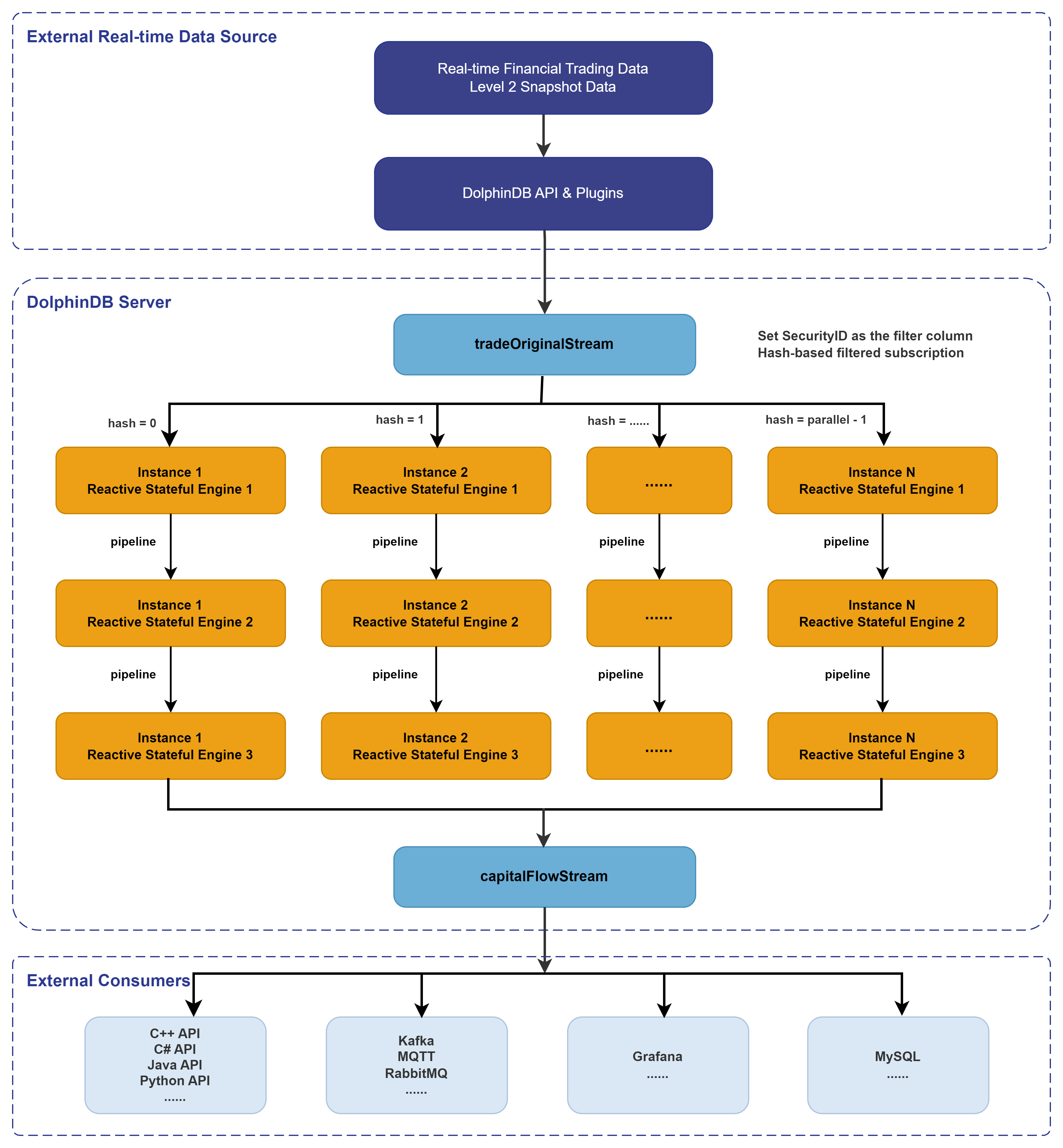
The diagram above illustrates the processing workflow:
-
tradeOriginalStream is a stream table in DolphinDB. It receives data from the real-time data source and publishes the data to the streaming engine for real-time calculation.
-
capitalFlowStream is a stream table in DolphinDB. It receives calculation results from the streaming engine in real time, and its data can be subscribed to and consumed by external consumers.
-
The parallel parameter specifies the parallelism of stream processing. In this tutorial, data in the tick-by-tick trade table tradeOriginalStream is distributed by hashing the SecurityID field (stock code) as evenly as possible across parallel reactive stateful engine 1 instances for parallel computation. Because the tick-by-tick trade table carries a large data volume and the daily cumulative order-by-order capital flow indicators are relatively complex to calculate, parallel stream processing is required.
-
Reactive stateful engine 1 uses the built-in
cumsumandprevfunctions to incrementally calculate the current order's cumulative trading value after grouping by stock code and buy order ID, as well as the order-size labels and cumulative trading volume before and after the current order is merged. The detailed calculation logic is explained in Chapter2. -
Reactive stateful engine 2 uses the built-in
cumsumandprevfunctions to incrementally calculate the current order's cumulative trading value after grouping by stock code and sell order ID, as well as the order-size labels and cumulative trading volume before and after the current order is merged. It also retains the intermediate buy-side calculation results from the previous step. The detailed calculation logic is explained in Chapter2. -
Reactive stateful engine 3 uses the built-in
cumsum,dynamicGroupCumsum, anddynamicGroupCumcountfunctions to incrementally calculate capital flow indicators aggregated by stock code. The detailed calculation logic is explained in Chapter2.
2. Daily Cumulative Capital Flow Indicator Implementation
2.1. Create Stream Tables
def createStreamTableFunc(){
	//create stream table: tradeOriginalStream
	colName = `SecurityID`Market`TradeTime`TradePrice`TradeQty`TradeAmount`BuyNum`SellNum
	colType = [SYMBOL, SYMBOL, TIMESTAMP, DOUBLE, INT, DOUBLE, INT, INT]
	tradeOriginalStreamTemp = streamTable(20000000:0, colName, colType)
	try{ enableTableShareAndPersistence(table=tradeOriginalStreamTemp, tableName="tradeOriginalStream", asynWrite=true, compress=true, cacheSize=20000000, retentionMinutes=1440, flushMode=0, preCache=10000) }
	catch(ex){ print(ex) }
	undef("tradeOriginalStreamTemp")

	//create stream table: capitalFlowStream
	colName = `SecurityID`TradeTime`TotalAmount`SellSmallAmount`SellMediumAmount`SellBigAmount`SellSmallCount`SellMediumCount`SellBigCount`BuySmallAmount`BuyMediumAmount`BuyBigAmount`BuySmallCount`BuyMediumCount`BuyBigCount
	colType = [SYMBOL, TIMESTAMP, DOUBLE, DOUBLE, DOUBLE, DOUBLE, INT, INT, INT, DOUBLE, DOUBLE, DOUBLE, INT, INT, INT]
	capitalFlowStreamTemp = streamTable(20000000:0, colName, colType)
	try{ enableTableShareAndPersistence(table=capitalFlowStreamTemp, tableName="capitalFlowStream", asynWrite=true, compress=true, cacheSize=20000000, retentionMinutes=1440, flushMode=0, preCache=10000) }
	catch(ex){ print(ex) }
	undef("capitalFlowStreamTemp")

	//create stream table: capitalFlowStream60min
	colName = `TradeTime`SecurityID`TotalAmount`SellSmallAmount`SellMediumAmount`SellBigAmount`SellSmallCount`SellMediumCount`SellBigCount`BuySmallAmount`BuyMediumAmount`BuyBigAmount`BuySmallCount`BuyMediumCount`BuyBigCount
	colType = [TIMESTAMP, SYMBOL, DOUBLE, DOUBLE, DOUBLE, DOUBLE, INT, INT, INT, DOUBLE, DOUBLE, DOUBLE, INT, INT, INT]
	capitalFlowStream60minTemp = streamTable(1000000:0, colName, colType)
	try{ enableTableShareAndPersistence(table=capitalFlowStream60minTemp, tableName="capitalFlowStream60min", asynWrite=true, compress=true, cacheSize=1000000, retentionMinutes=1440, flushMode=0, preCache=10000) }
	catch(ex){ print(ex) }
	undef("capitalFlowStream60minTemp")
}

createStreamTableFunc()
go
setStreamTableFilterColumn(tradeOriginalStream, `SecurityID)-
The
gostatement parses and executes code in segments. -
The
setStreamTableFilterColumnfunction specifies the filter column for a stream table and is used together with the filter parameter ofsubscribeTable. In this tutorial, it distributes data in the tick-by-tick trade table by hashing stock codes as evenly as possible across different stream processing threads, enabling parallel computation.
2.2. Define a Function for Capital Flow Order-Size Classification
/** Label small, medium, and large orders
* small: 0
* medium: 1
* large: 2*/
@state
def tagFunc(qty){
 return iif(qty <= 20000, 0, iif(qty <= 200000 and qty > 20000, 1, 2))
}-
Orders with trading volume less than or equal to 20,000 shares are classified as small orders and labeled 0; orders with trading volume greater than 20,000 shares and less than or equal to 200,000 shares are classified as medium orders and labeled 1; orders with trading volume greater than 200,000 shares are classified as large orders and labeled 2. In this tutorial, capital flow order-size classification is based on the number of shares traded. Orders are divided into large, medium, and small categories. The threshold values are user-defined, and you must adjust them for your specific use cases.
-
Because this function is used in the reactive stateful engine, you must add
@stateto declare that it is a stateful function before the definition.
2.3. Incremental Calculation Grouped by Stock and Buy order ID
def processBuyOrderFunc(parallel){
	metricsBuy = [
		<TradeTime>,
		<SellNum>,
		<TradeAmount>,
		<TradeQty>,
		<cumsum(TradeAmount)>,
		<tagFunc(cumsum(TradeQty))>,
		<prev(cumsum(TradeAmount))>,
		<prev(tagFunc(cumsum(TradeQty)))>]
	for(i in 1..parallel){
		createReactiveStateEngine(name="processBuyOrder"+string(i), metrics=metricsBuy, dummyTable=tradeOriginalStream, outputTable=getStreamEngine("processSellOrder"+string(i)), keyColumn=`SecurityID`BuyNum, keepOrder=true)
		subscribeTable(tableName="tradeOriginalStream", actionName="processBuyOrder"+string(i), offset=-1, handler=getStreamEngine("processBuyOrder"+string(i)), msgAsTable=true, hash=i, filter=(parallel, i-1))
	}
}-
The parallel parameter specifies the degree of parallelism. In the preceding code, the data in the tick-by-tick trade table tradeOriginalStream is hash-partitioned by stock symbol and distributed as evenly as possible across the number of reactive stateful engine instances specified by parallel. These instances use the same computation logic but process different sets of stocks.
-
The preceding code uses DolphinDB's reactive stateful engine and the built-in
cumsumandprevfunctions to perform streaming incremental computation. The grouping fields are SecurityID and BuyNum, that is, the stock code and buy order ID. -
metricsBuy contains the calculation formulas represented as metacode in the reactive stateful engine:
metricsBuy = [
 	<TradeTime>,
 	<SellNum>,
 	<TradeAmount>,
 	<TradeQty>,
 	<cumsum(TradeAmount)>,
 	<tagFunc(cumsum(TradeQty))>,
 	<prev(cumsum(TradeAmount))>,
<prev(tagFunc(cumsum(TradeQty)))>]<TradeTime>, <SellNum>, <TradeAmount>, <TradeQty> are stateless calculations. They preserve the original values of these fields from the source table and pass them to the next layer of reactive stateful engines for computation. <cumsum(TradeAmount)>, <tagFunc(cumsum(TradeQty))>, <prev(cumsum(TradeAmount))>, <prev(tagFunc(cumsum(TradeQty)))> are stateful calculations. For each trade record, they calculate:
-
the cumulative trading value aggregated by the buy order ID to which the current trade belongs;
-
the order-size label determined from the cumulative traded volume after the current trade is incorporated;
-
the cumulative trading value before the current trade is incorporated; and
-
the order-size label determined from the cumulative traded volume before the current trade is incorporated.
These stateful results serve as inputs to the dynamicGroupCumsum and dynamicGroupCumcount functions in the third-layer reactive stateful engine, enabling incremental computation of buy-side capital flow indicators.
All of these stateful factors are computed incrementally in a streaming manner.
To illustrate the computation logic, the following example feeds sample data into the first-layer reactive stateful engine and shows how it processes each input:
-
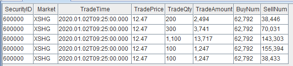
Write five records to the tick-by-tick trades table tradeOriginalStream:
-
After processing by the first-layer reactive stateful engine, the output is as follows:

The preceding code performs merged calculations on tick-by-tick trades for stock code 60000 by buy order ID 69792. Because the reactive stateful engine performs a reactive calculation for each input record, the number of output records is the same as the number of input records. In the result table, TotalBuyAmount, BuyOrderFlag, PrevTotalBuyAmount, and PrevBuyOrderFlag represent, respectively, the cumulative trading value after each trade record is merged by the buy order ID for the corresponding stock, the order-size label determined by the cumulative trading volume after the current record is merged, the cumulative trading value before the current record is merged, and the order-size label determined by the cumulative trading volume before the current record is merged. All of these stateful factors are calculated through streaming incremental computation.
2.4. Incremental Calculation Grouped by Stock and Sell Order ID
def processSellOrderFunc(parallel){
	colName = `SecurityID`BuyNum`TradeTime`SellNum`TradeAmount`TradeQty`TotalBuyAmount`BuyOrderFlag`PrevTotalBuyAmount`PrevBuyOrderFlag
	colType = [SYMBOL, INT, TIMESTAMP, INT, DOUBLE, INT, DOUBLE, INT, DOUBLE, INT]
	processBuyOrder = table(1:0, colName, colType)
	metricsSell = [
		<TradeTime>,
		<TradeAmount>,
		<cumsum(TradeAmount)>,
		<tagFunc(cumsum(TradeQty))>,
		<prev(cumsum(TradeAmount))>,
		<prev(tagFunc(cumsum(TradeQty)))>,
		<BuyNum>,
		<TotalBuyAmount>,
		<BuyOrderFlag>,
		<PrevTotalBuyAmount>,
		<PrevBuyOrderFlag>]
	for(i in 1..parallel){
		createReactiveStateEngine(name="processSellOrder"+string(i), metrics=metricsSell, dummyTable=processBuyOrder, outputTable=getStreamEngine("processCapitalFlow"+string(i)), keyColumn=`SecurityID`SellNum, keepOrder=true)
	}
}-
The parallel parameter specifies the parallelism of stream computing. In the preceding code, parallel instances of reactive stateful engine 2 are created. Each instance receives the output of its corresponding first-layer reactive stateful engine, enabling parallel processing. All second-layer reactive stateful engine instances execute the same computation logic but process different sets of stocks.
-
The preceding code uses DolphinDB's reactive stateful engine and the built-in
cumsumandprevfunctions to perform streaming incremental computation. The grouping fields are SecurityID and SellNum, that is, the stock code and sell order ID. -
metricsSell contains the calculation formulas represented as metacode in the reactive stateful engine:
metricsSell = [
 	<TradeTime>,
 	<TradeAmount>,
 	<cumsum(TradeAmount)>,
 	<tagFunc(cumsum(TradeQty))>,
 	<prev(cumsum(TradeAmount))>,
 	<prev(tagFunc(cumsum(TradeQty)))>,
 	<BuyNum>,
 	<TotalBuyAmount>,
 	<BuyOrderFlag>,
 	<PrevTotalBuyAmount>,
<PrevBuyOrderFlag>]<TradeTime>, <TradeAmount>, <BuyNum>, <TotalBuyAmount>, <BuyOrderFlag>, <PrevTotalBuyAmount>, <PrevBuyOrderFlag> are stateless calculations. They preserve the original values of these fields from the source table and pass them to the next layer of reactive stateful engines for computation. <cumsum(TradeAmount)>, <tagFunc(cumsum(TradeQty))>, <prev(cumsum(TradeAmount))>, <prev(tagFunc(cumsum(TradeQty)))> are stateful calculations. For each trade record, they calculate:
-
the cumulative trading value aggregated by the sell order ID to which the current trade belongs;
-
the order-size label determined from the cumulative traded volume after including the current trade;
-
the cumulative trading value before including the current trade; and
-
the order-size label determined from the cumulative traded volume before including the current trade.
These results are used as inputs to the dynamicGroupCumsum and dynamicGroupCumcount functions in the third-layer reactive stateful engine to incrementally calculate sell-side capital flow indicators. All of these stateful factors are calculated through streaming incremental computation.
To better illustrate the computation logic of this section, the following example uses sample data to demonstrate how the second-layer reactive stateful engine works.
-
The input to the second-layer reactive stateful engine is as follows:
-
After processing by the second-layer reactive stateful engine, the output is as follows:

The preceding code performs merged calculations on tick-by-tick trades for stock code 60000 by sell order IDs 38446, 70031, 143303, 155394, and 38433. Because the reactive stateful engine performs a reactive calculation for each input record, the number of output records is the same as the number of input records. In the result table, TotalSellAmount, SellOrderFlag, PrevTotalSellAmount, and PrevSellOrderFlag represent, respectively, the cumulative trading value after each trade record is merged by the sell order ID for the corresponding stock, the order-size label determined by the cumulative trading volume after the current record is merged, the cumulative trading value before the current record is merged, and the order-size label determined by the cumulative trading volume before the current record is merged. All of these stateful factors are calculated through streaming incremental computation.
2.5. Incremental Calculation of Capital Flow Indicators Grouped by Stock
def processCapitalFlowFunc(parallel){
	colName = `SecurityID`SellNum`TradeTime`TradeAmount`TotalSellAmount`SellOrderFlag`PrevTotalSellAmount`PrevSellOrderFlag`BuyNum`TotalBuyAmount`BuyOrderFlag`PrevTotalBuyAmount`PrevBuyOrderFlag
	colType = [SYMBOL, INT, TIMESTAMP, DOUBLE, DOUBLE, INT, DOUBLE, INT, INT, DOUBLE, INT, DOUBLE, INT]
	processSellOrder = table(1:0, colName, colType)
	metrics1 = <dynamicGroupCumsum(TotalSellAmount, PrevTotalSellAmount, SellOrderFlag, PrevSellOrderFlag, 3)>
	metrics2 = <dynamicGroupCumcount(SellOrderFlag, PrevSellOrderFlag, 3)>
	metrics3 = <dynamicGroupCumsum(TotalBuyAmount, PrevTotalBuyAmount, BuyOrderFlag, PrevBuyOrderFlag, 3)>
	metrics4 = <dynamicGroupCumcount(BuyOrderFlag, PrevBuyOrderFlag, 3)>
	for(i in 1..parallel){
		createReactiveStateEngine(name="processCapitalFlow"+string(i), metrics=[<TradeTime>, <cumsum(TradeAmount)>, metrics1, metrics2, metrics3, metrics4], dummyTable=processSellOrder, outputTable=capitalFlowStream, keyColumn=`SecurityID, keepOrder=true)
	}
}-
In the preceding code, parallel instances of reactive stateful engine 3 are created. Each instance takes the output of the corresponding one of the parallel instances of reactive stateful engine 2 as input to perform parallel computation. These reactive stateful engine 3 instances use the same computation logic but process different stocks.
-
The preceding code uses DolphinDB's reactive stateful engine and the built-in
cumsum,dynamicGroupCumsum, anddynamicGroupCumcountfunctions to implement streaming incremental computation. The grouping field is SecurityID, which is the stock code. -
metrics contains the calculation formulas represented as metacode in the reactive stateful engine:
metrics1 = <dynamicGroupCumsum(TotalSellAmount, PrevTotalSellAmount, SellOrderFlag, PrevSellOrderFlag, 3)>
metrics2 = <dynamicGroupCumcount(SellOrderFlag, PrevSellOrderFlag, 3)>
metrics3 = <dynamicGroupCumsum(TotalBuyAmount, PrevTotalBuyAmount, BuyOrderFlag, PrevBuyOrderFlag, 3)>
metrics4 = <dynamicGroupCumcount(BuyOrderFlag, PrevBuyOrderFlag, 3)>
metrics = [<TradeTime>, <cumsum(TradeAmount)>, metrics1, metrics2, metrics3, metrics4]
<TradeTime> is a stateless calculation that preserves the original timestamp for each calculation result.
<cumsum(TradeAmount)> is a stateful calculation that represents the stock's total trading value from market open to the current tick.
In metrics1, <dynamicGroupCumsum(TotalSellAmount, PrevTotalSellAmount, SellOrderFlag, PrevSellOrderFlag, 3)> is a stateful calculation. Its inputs are the cumulative trading value for the stock represented by the current trade record after merging by the record's sell order ID, the cumulative trading value before the current trade record is merged, the order-size label determined from cumulative trading volume after the current trade record is merged, the order-size label determined from cumulative trading volume before the current trade record is merged, and the number of order-size labels. Its outputs are the stock's total trading value for small sell orders, medium sell orders, and large sell orders from market open to the current tick.
In metrics2, <dynamicGroupCumcount(SellOrderFlag, PrevSellOrderFlag, 3)> is a stateful calculation. Its inputs are the order-size label determined from cumulative trading volume after the stock represented by the current trade record is merged by the record's sell order ID, the order-size label determined from cumulative trading volume before the current trade record is merged, and the number of order-size labels. Its outputs are the stock's total number of small sell orders, medium sell orders, and large sell orders from market open to the current tick.
metrics3 and metrics4 are also stateful calculations. They represent buy-side capital flow indicators and use logic similar to the sell-side calculations, so they are not described in detail here.
All of these stateful factors are calculated through streaming incremental computation.
To better understand the computation logic of this section, let's use some sample data to observe how the third-layer reactive stateful engine processes the data.
-
The input to the third-layer reactive stateful engine is
-
After processing by the third-layer reactive stateful engine, the output is

The preceding figure shows the calculation results for daily cumulative order-by-order capital flow indicators for the stock code 60000. In a reactive stateful engine, each input record triggers one reactive calculation, so the number of output results equals the number of input records.
In the result table, TotalAmount represents the stock's total trading value from market open to the current tick. The calculation expression is <cumsum(TradeAmount)>, and the input is the trading value of each trade. Streaming incremental computation is implemented through the reactive stateful engine and the cumsum cumulative sum function.
In the result table, SellSmallAmount, SellMediumAmount, and SellBigAmount represent the stock's total trading value for small sell orders, medium sell orders, and large sell orders from market open to the current tick. The calculation expression is <dynamicGroupCumsum(TotalSellAmount, PrevTotalSellAmount, SellOrderFlag, PrevSellOrderFlag, 3)>. The inputs are the cumulative trading value for the stock represented by the current trade record after merging by the record's sell order ID, the cumulative trading value before the current trade record is merged, the order-size label determined from cumulative trading volume after the current trade record is merged, the order-size label determined from cumulative trading volume before the current trade record is merged, and the number of order-size labels. Streaming incremental computation is implemented through the reactive stateful engine and the dynamicGroupCumsum function. In real-time daily cumulative capital flow calculation, as trading volume continues to increase, an order may change from a small order to a large order. In that case, the value already accumulated for the order must be subtracted from the cumulative statistic for small orders, and the latest cumulative value of the order must be added to the cumulative statistic for large orders. The dynamicGroupCumsum function applies to this type of scenario.
In the result table, SellSmallCount, SellMediumCount, and SellBigCount represent the stock's total number of small sell orders, medium sell orders, and large sell orders from market open to the current tick. The calculation expression is <dynamicGroupCumcount(SellOrderFlag, PrevSellOrderFlag, 3)>. The inputs are the order-size label determined from cumulative trading volume after the stock represented by the current trade record is merged by the record's sell order ID, the order-size label determined from cumulative trading volume before the current trade record is merged, and the number of order-size labels. Streaming incremental computation is implemented through the reactive stateful engine and the dynamicGroupCumcount function. In real-time daily cumulative capital flow calculation, as trading volume continues to increase, an order may change from a small order to a large order. In that case, the cumulative statistic for small orders must be decremented by 1, and the cumulative statistic for large orders must be incremented by 1. The dynamicGroupCumcount function applies to this type of scenario.
In the result table, BuySmallAmount, BuyMediumAmount, BuyBigAmount, BuySmallCount, BuyMediumCount, and BuyBigCount represent buy-side daily cumulative capital flow indicators. Their computation logic is similar to that of the sell-side indicators and is not described in detail here. Streaming incremental computation is also implemented through the reactive stateful engine and the dynamicGroupCumsum and dynamicGroupCumcount functions.
2.6. Push Calculation Results at a Fixed Frequency
def processCapitalFlow60minFunc(){
	aggrMetrics = <[
		last(TotalAmount),
		last(SellSmallAmount),
		last(SellMediumAmount),
		last(SellBigAmount),
		last(SellSmallCount),
		last(SellMediumCount),
		last(SellBigCount),
		last(BuySmallAmount),
		last(BuyMediumAmount),
		last(BuyBigAmount),
		last(BuySmallCount),
		last(BuyMediumCount),
		last(BuyBigCount)]>
	createDailyTimeSeriesEngine(name="processCapitalFlow60min", windowSize=60000*60, step=60000*60, metrics=aggrMetrics, dummyTable=capitalFlowStream, outputTable=capitalFlowStream60min, timeColumn="TradeTime", useSystemTime=false, keyColumn=`SecurityID, useWindowStartTime=false)
	subscribeTable(tableName="capitalFlowStream", actionName="processCapitalFlow60min", offset=-1, handler=getStreamEngine("processCapitalFlow60min"), msgAsTable=true, batchSize=10000, throttle=1, hash=0)
}-
The grouping field is SecurityID, which is the stock code.
-
Use DolphinDB's time-series engine to perform real-time 60-minute rolling window calculations on the capital flow indicator result table. The aggregate function is
last. -
The data source for real-time calculation is the daily cumulative capital flow result table, capitalFlowStream. Although this table has high data throughput, matching that of the original tick-by-tick trades table, it performs only simple 60-minute rolling indicator calculations, so single-threaded processing is sufficient and parallel stream processing is not required.
2.7. Register the Subscription Engine and Subscribe to Stream Tables
parallel = 3
processCapitalFlowFunc(parallel)
go
processSellOrderFunc(parallel)
go
processBuyOrderFunc(parallel)
processCapitalFlow60minFunc()
This tutorial sets parallel=3, which means the capital flow
calculation runs with a parallelism of 3 and can support a maximum upstream
tick-by-tick trade data throughput of 50,000 records per second. On a day in
January 2022, the peak throughput of tick-by-tick trade data for all stocks on
the Shanghai and Shenzhen exchanges reached 42,000 records per second at the
09:30:00 market open. Therefore, in production deployment, to prevent increased
latency caused by stream processing backlogs during traffic peaks, you can set
parallel to 3 to increase the system's maximum real-time computation
capacity.
2.8. Replay Historical Data
//replay historical data
t = select * from loadTable("dfs://trade", "trade") where time(TradeTime) between 09:30:00.000: 15:00:00.000 order by TradeTime, SecurityID
submitJob("replay_trade", "trade", replay{t, tradeOriginalStream, `TradeTime, `TradeTime, 50000, true, 1})
getRecentJobs()
After execution, the function returns the following information:

If endTime and errorMsg are empty, the task is running normally.
3. Display Real-Time Daily Cumulative Capital Flow Calculation Results
3.1. In-Node Calculation Result Table
The calculation result table capitalFlowStream can be queried in real time through any DolphinDB API query interface. You can also view the table results in real time in the DolphinDB GUI. The result is:

3.2. Push Calculation Results at a Fixed Frequency
The result table capitalFlowStream contains the same number of records as the tick-by-tick trade data, with one response generated for each trade record.
To periodically obtain a cross-sectional snapshot of the latest daily cumulative capital flow indicators for each stock, use DolphinDB's built-in time-series engine to retrieve the last record for each stock at the end of each fixed time window. In this tutorial, real-time rolling-window calculations are performed on the result table capitalFlowStream. The window size is 60 minutes, and the results are stored in the capitalFlowStream60min stream table. The data is shown in the following figure:

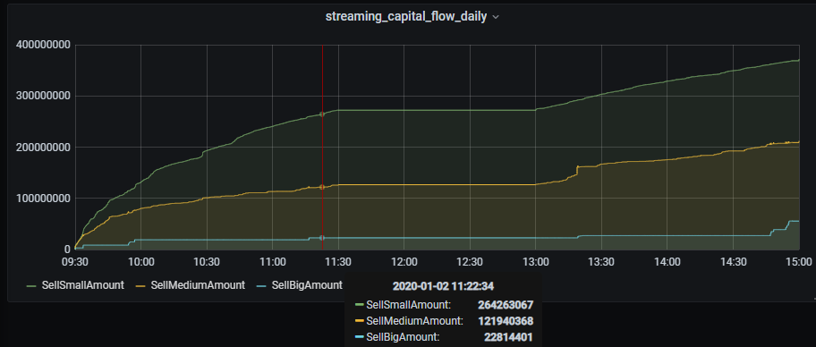
3.3 . Real-Time Result Monitoring in Grafana
DolphinDB integrates with Grafana for real-time visualization of streaming results. After connecting Grafana to the DolphinDB data source, you can build dashboards that display live capital flow indicators as they are computed.
The dashboard above shows daily cumulative capital flow indicators — including trading value, buy/sell-side amounts by order size, and order counts — updated continuously as new trade data flows through the pipeline.
4. Performance Testing
This tutorial tests two scenarios: single-response calculation and continuous-response calculation. The test data consists of tick-by-tick trade data for 1,558 stocks on a trading day in 2020 on the Shanghai Stock Exchange.
Development Environment
-
CPU: Intel(R)Xeon(R)Silver 4216 CPU@2.10GHz
-
Total logical CPU cores: 8
-
Memory: 64 GB
-
OS: 64-bit CentOS Linux 7 (Core)
-
Disk: SSD, with a maximum read/write speed of 520 MB/s
-
Server versions: 1.30.18, 2.00.6
4.1. Performance Test for Single-Response Calculation
This tutorial uses a pipeline of three chained reactive stateful engines. The end-to-end response time is measured from when the first engine receives input to when the third engine outputs the result. The test measures the performance of a single pass for 1 stock and for 1,558 stocks respectively. The total elapsed time for 10 runs was recorded, and the average was used as the elapsed time for a single run. The single-threaded test results are as follows:
Table 1-1 Test Results
| Number of Stocks | Elapsed Time (ms) |
|---|---|
| 1 | 0.18 |
| 1,558 | 2.09 |
4.2. Performance Test for Continuous-Response Calculation
This tutorial uses a pipeline of three chained reactive stateful engines. With a pipeline parallelism of 3, it can sustain a maximum upstream tick-by-tick throughput of 50,000 records per second. Using 16.32 million tick-by-tick trade records for 1,558 stocks on a trading day in 2020 on the Shanghai Stock Exchange as the test data, DolphinDB's replay function replays historical data and ingests it as streaming data into the upstream stream table tradeOriginalStream. The replay runs at full speed. The total calculation time is 326 seconds, for a processing capacity of 50,000 records per second. You can increase the parallelism to improve system throughput.
5. Appendix
-
Clear environment and create required stream table: 01.createStreamTB.txt
-
Create streaming engine and subscribe to stream table: 02.createEngineSub.txt
-
Replay historical data: 03.replay.txt
-
Functions for monitoring stream processing: 04.streamStateQuery.txt
-
Test data: 20200102_SH_trade.csv