Time Bucket Engine
Overview
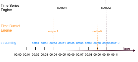
Similar to the time-series engine, the time bucket engine can partition data based on a specified time window and perform aggregation within each window. The difference is that the time-series engine can only aggregate over fixed-length windows, and the aggregation is triggered when the first timestamp exceeds the window’s right boundary. In contrast, the time bucket engine allows custom definitions of time windows and triggers aggregation immediately when the window closes. This engine is suitable for scenarios requiring real-time computation over variable-length windows. When used in combination with a time-series engine, it can further process high-frequency aggregation results, such as:
-
Generate 5-minute, 15-minute, or 30-minute OHLC bars from existing 1-minute OHLC bars.
-
Generate factors in 5-minute, 15-minute, or 30-minute frequency from existing factors in 1-minute frequency, based on user-defined logic.
For example, generate 5-minute OHLC bars from 1-minute OHLC bars. The raw market data is first processed by the time-series engine to generate 1-minute OHLC data, which is then fed into the time bucket engine. Within a 5-minute window [09:00, 09:05), when a 1-minute OHLC bar is input, if its timestamp reaches or exceeds the window’s right boundary (09:04), the time bucket engine immediately closes the window and performs the computation. If the time-series engine is used again to generate 5-minute OHLC bars, it must wait for data at 09:05 or later to produce the output.
The time bucket engine is created using the createTimeBucketEngine
function.
Syntax:
createTimeBucketEngine(name,timeCutPoints,metrics,dummyTable,outputTable,timeColumn,[keyColumn],[useWindowStartTime],[closed='left'],[fill='none'],[keyPurgeFreqInSec=-1],[outputElapsedMicroseconds=false],[parallelism=1],[outputHandler=NULL],[msgAsTable=false],[snapshotDir],[snapshotIntervalInMsgCount])
For parameter description, see createTimeBucketEngine.
Examples
The following example demonstrates how the time bucket engine aligns window boundaries and performs window-based aggregation by generating 5-minute OHLC bars from 1-minute OHLC bars.
First, create a stream table named trades with four columns (time, sym, price, and volume) to simulate a stock market data source. Then create a time-series engine named timeSeries1 to generate 1-minute OHLC data based on data from the trades table, and write the results to the stream table named output1.
share streamTable(1000:0, `time`sym`price`volume, [TIMESTAMP, SYMBOL, DOUBLE, INT]) as trades
share streamTable(1000:0, `time`sym`firstPrice`maxPrice`minPrice`lastPrice`sumVolume, [TIMESTAMP, SYMBOL, DOUBLE, DOUBLE, DOUBLE, DOUBLE, INT]) as output1
timeSeries1 = createTimeSeriesEngine(name="timeSeries1", windowSize=60000, step=60000, metrics=<[first(price), max(price), min(price), last(price), sum(volume)]>, dummyTable=trades, outputTable=output1, timeColumn=`time, useSystemTime=false, keyColumn=`sym, useWindowStartTime=false)
subscribeTable(tableName="trades", actionName="timeSeries1", offset=0, handler=append!{timeSeries1}, msgAsTable=true)
Next, create a time bucket engine named timeBucket1. By subscribing to the output1 table, the 1-minute OHLC data is fed into timeBucket1 to generate 5-minute OHLC data, and the results are written to the output2 table. In timeCutPoints, any two adjacent elements define the left and right boundaries of a window. The time precision of the elements in timeCutPoints determines the precision of the right boundary when the window is closed.
output2 = table(1000:0, `time`sym`firstPrice`maxPrice`minPrice`lastPrice`sumVolume, [TIMESTAMP, SYMBOL, DOUBLE, DOUBLE, DOUBLE, DOUBLE, INT])
timeCutPoints=[10:00m, 10:05m, 10:10m, 10:15m]
timeBucket1 = createTimeBucketEngine(name="timeBucket1", timeCutPoints=timeCutPoints, metrics=<[first(firstPrice), max(maxPrice), min(minPrice), last(lastPrice), sum(sumVolume)]>, dummyTable=output1, outputTable=output2, timeColumn=`time, keyColumn=`sym)
subscribeTable(tableName="output1", actionName="timeBucket1", offset=0, handler=append!{timeBucket1}, msgAsTable=true);
Insert data into the trades table.
insert into trades values(2024.10.08T10:01:01.785,`A, 10.83, 2110)
insert into trades values(2024.10.08T10:01:02.125,`B,21.73, 1600)
insert into trades values(2024.10.08T10:01:12.457,`A,10.79, 2850)
insert into trades values(2024.10.08T10:03:10.789,`A,11.81, 2250)
insert into trades values(2024.10.08T10:03:12.005,`B, 22.96, 1980)
insert into trades values(2024.10.08T10:08:02.236,`A, 11.25, 2400)
insert into trades values(2024.10.08T10:08:04.412,`B, 23.03, 2130)
insert into trades values(2024.10.08T10:08:05.152,`B, 23.18, 1900)
insert into trades values(2024.10.08T10:08:30.021,`A, 11.04, 2300)
insert into trades values(2024.10.08T10:09:20.123,`A, 11.85, 2200)
insert into trades values(2024.10.08T10:10:02.236,`A, 11.06, 2200)
insert into trades values(2024.10.08T10:11:04.412,`B, 23.15, 1880)
View the results output by the timeSeries1 engine.
select * from output1| time | sym | firstPrice | maxPrice | minPrice | lastPrice | sumVolume |
|---|---|---|---|---|---|---|
| 2024.10.08 10:02:00.000 | A | 10.83 | 10.83 | 10.79 | 10.79 | 4,960 |
| 2024.10.08 10:02:00.000 | B | 21.73 | 21.73 | 21.73 | 21.73 | 1,600 |
| 2024.10.08 10:04:00.000 | A | 11.81 | 11.81 | 11.81 | 11.81 | 2,250 |
| 2024.10.08 10:04:00.000 | B | 22.96 | 22.96 | 22.96 | 22.96 | 1,980 |
| 2024.10.08 10:09:00.000 | A | 11.25 | 11.25 | 11.04 | 11.04 | 4,700 |
| 2024.10.08 10:09:00.000 | B | 23.03 | 23.18 | 23.03 | 23.18 | 4,030 |
| 2024.10.08 10:10:00.000 | A | 11.85 | 11.85 | 11.85 | 11.85 | 2,200 |
The time bucket engine determines the time range based on the first and last elements in timeCutPoints. Within a time window, the window is closed when the engine receives the first record whose timestamp is greater than or equal to the right boundary of that window. The data within the window is then aggregated according to the rules defined in the metrics parameter. The time precision of the engine is also determined by the time precision of timeCutPoints. If the time vector in timeCutPoints has minute-level precision, the engine partitions windows and performs computation at the minute level. If the precision is at the second level, the engine works at the second level.
In this example, the time bucket engine performs grouped computation based on the grouping column sym, specified by the keyColumn parameter. Since groups A and B follow the same computation logic, we only explain group A. The first record of group A has a timestamp of 10:02:00.000 (hereafter referred to as 10:02m), which falls within the first window [10:00m, 10:05m). When the window boundary is left-closed and right-open, the window closes when the engine receives data whose timestamp is greater than or equal to the right boundary minus one time unit. Therefore, when data with a timestamp greater than or equal to 10:04m is inserted, the window closes. The engine then aggregates the data at 10:02m and 10:04m within that window according to the metrics rules and outputs the result. When data at 10:09m is inserted, the window [10:05m, 10:10m) closes at 10:09m. Since there is only one record in this window, the aggregation result is based on that single record. After the 10:10m record of group A is inserted, the window does not close because data with a timestamp greater than or equal to 10:14m has not yet arrived. Therefore, no aggregation is performed at that time.
Next, we demonstrate the computation results when the window boundary is left-open and right-closed. Create a time bucket engine named timeBucket2, specify the window boundary as left-open and right-closed using the closed parameter, subscribe to the output1 table, and write the results to the output3 table.
output3 = table(1000:0, `time`sym`firstPrice`maxPrice`minPrice`lastPrice`sumVolume, [TIMESTAMP, SYMBOL, DOUBLE, DOUBLE, DOUBLE, DOUBLE, INT])
timeBucket2 = createTimeBucketEngine(name="timeBucket2", timeCutPoints=timeCutPoints, metrics=<[first(firstPrice), max(maxPrice), min(minPrice), last(lastPrice), sum(sumVolume)]>, dummyTable=output1, outputTable=output3, timeColumn=`time, keyColumn=`sym, closed='right')
subscribeTable(tableName="output1", actionName="timeBucket2", offset=0, handler=append!{timeBucket2}, msgAsTable=true);
View the results output by the timeSeries1 engine.
select * from output3| time | sym | firstPrice | maxPrice | minPrice | lastPrice | sumVolume |
|---|---|---|---|---|---|---|
| 2024.10.08 10:05:00.000 | A | 10.83 | 11.81 | 10.79 | 11.81 | 7,210 |
| 2024.10.08 10:05:00.000 | B | 21.73 | 22.96 | 21.73 | 22.96 | 3,580 |
| 2024.10.08 10:10:00.000 | A | 11.25 | 11.85 | 11.04 | 11.85 | 6,900 |
When the window boundary is left-open and right-closed, the window is closed when the first record with a timestamp greater than or equal to the right boundary is inserted. In this example, when the first record whose timestamp is greater than or equal to the right boundary of the interval (10:00m, 10:05m] arrives (that is, the record at 10:09m), the window closes. The engine then aggregates the data at 10:02m and 10:04m and outputs the result. After the 10:10m record of group A is inserted, the window (10:05m, 10:10m] closes, and the engine aggregates the data at 10:09m and 10:10m.
Related functions