Reactive Stateless Engine
The reactive stateless engine is designed to handle the dependencies within data streams. When the value of one data item depends on the latest state of one or more data items, the engine ensures that whenever any upstream dependency changes, all results that depend on it, whether directly or indirectly, are automatically recalculated and output in real time. The overall workflow is similar to triggering recalculation in Excel.
For example, the price of a derivative instrument (such as an option) may depend on the factors of the underlying asset, such as the latest price, volatility, and other indicators. Whenever any of these indicators change, the derivative price needs to be recalculated immediately.
If you define functions to calculate these indicators, maintaining a dependency graph can be challenging, especially when the relationships among the metrics are complex (e.g., Indicator A affects Indicator B, and Indicator B affects Indicator C). With the reactive stateless engine, you do not need to manually build or maintain a dependency graph, nor write trigger logic or state propagation code. You simply define the calculation rules using declarative syntax, and the system will automatically, efficiently, and reliably handle data flow and calculations. This not only significantly improves development efficiency and reduces code complexity and the risk of errors, but also provides highly optimized, high-performance computing capabilities that integrate seamlessly with stream processing frameworks, offering an out-of-the-box experience.
The reactive stateless engine is created via
createReactiveStatelessEngine. The syntax is as follows:
createReactiveStatelessEngine(name, metrics, outputTable, [snapshotDir], [snapshotIntervalInMsgCount])
See createReactiveStatelessEngine for details.
Calculation Rules
The reactive stateless engine processes each batch of input data and calculates formulas as defined in metrics. Once a precedent value (referred to by a metric) is ingested or updated, all dependent formulas are output accordingly. The calculation is based on the latest variable values.
The following examples provide a step-by-step explanation of how to use the reactive stateless engine to monitor an investment portfolio's risk.
Usage Examples
Example 1. Update Total Stock Value in Real Time
The formula for calculating the total value of stock A is: Holding Value = Latest Price x Holding Quantity.
In Excel, it can be calculated by (amount= stock_A.price * stock_A.volume):
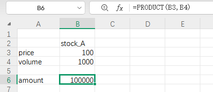
Use the reactive stateless engine to calculate:
// 1. Create the output table
outputTable = table(1:0, `product`metric`value, [STRING, STRING, DOUBLE])
// 2. Define dependencies (Metrics)
metrics = array(ANY, 0)
// Rule 1: Calculate the value of stock A
// The values in the engine are represented in the form of rowname:colname
metricA = dict(STRING, ANY)
metricA["outputName"] = `stock_A:`amount  // Represents the output result
metricA["formula"] = <price * volume> // Define the calculation formula, where price and volume are defined below
metricA["price"] = `stock_A:`price // Define the value of price
metricA["volume"] = `stock_A:`volume // Define the value of volume
metrics.append!(metricA)
// 3. Create the engine
engine = createReactiveStatelessEngine("portfolioEngine", metrics, outputTable)
// 4. Simulate data input
insert into engine values(["stock_A"],["price","volume"],[10])
insert into engine values(["stock_A"],["volume"],[1000])
// Or: insert into engine values(["stock_A","stock_A"],["price","volume"],[10,1000])
The output:
| product | metric | value |
|---|---|---|
| stock_A | amount | 10,000 |
Example 2. Update Total Portfolio Value in Real Time
In this section, we will build on Example 1 and demonstrate how to update the value of a single stock and the total portfolio value in real time. Using two stocks as an example, the formulas are as follows:
Holding Value of Stock A = Latest Price of Stock A × Holding Quantity of Stock A Holding Value of Stock B = Latest Price of Stock B × Holding Quantity of Stock B
Total Value of the Portfolio = Holding Value of Stock A + Holding Value of Stock B
try{dropStreamEngine("portfolioEngine")}catch(ex){}
// 1. Create the output table (using a keyed table, only keeping the latest state)
outputTable = keyedTable(`product`metric,1:0, `product`metric`value, [STRING, STRING, DOUBLE])
// 2. Define dependencies (Metrics)
metrics = array(ANY, 0)
// Rule 1: Calculate the holding value of stock A
metricA = dict(STRING, ANY)
metricA["outputName"] = `stock_A:`amount
metricA["formula"] = <price * volume>
metricA["price"] = `stock_A:`price
metricA["volume"] = `stock_A:`volume
metrics.append!(metricA)
// Rule 2: Calculate the holding value of stock B
metricB = dict(STRING, ANY)
metricB["outputName"] = `stock_B:`amount
metricB["formula"] = <price * volume>
metricB["price"] = `stock_B:`price
metricB["volume"] = `stock_B:`volume
metrics.append!(metricB)
// Rule 3: Calculate the total portfolio value (depends on the results of the first two rules)
metricAB = dict(STRING, ANY)
metricAB["outputName"] = `portfolio:`amount
metricAB["formula"] = <A_amount + B_amount>
metricAB["A_amount"] = `stock_A:`amount
metricAB["B_amount"] = `stock_B:`amount
metrics.append!(metricAB)
// 3. Create the engine
engine = createReactiveStatelessEngine("portfolioEngine", metrics, outputTable)
// 4. Simulate data input
insert into engine values("stock_A","price",10)
insert into engine values("stock_A","volume",1000)
insert into engine values("stock_B","price",20)
insert into engine values("stock_B","volume",1000)
The output:
| product | metric | value |
|---|---|---|
| stock_A | amount | 10,000 |
| stock_B | amount | 20,000 |
| portfolio | amount | 30,000 |
Example 3. Portfolio Risk Monitoring
The position value depends on the latest price and quantity, while the Value at Risk (VaR) further depends on the holding value and volatility. The total portfolio risk is then aggregated from the VaR of individual assets. Any updates to the underlying market data will automatically trigger the recalculation of all metrics directly or indirectly affected. This automated dependency propagation mechanism enables risk managers to continuously monitor the overall risk of the portfolio in real time and respond immediately to market fluctuations.
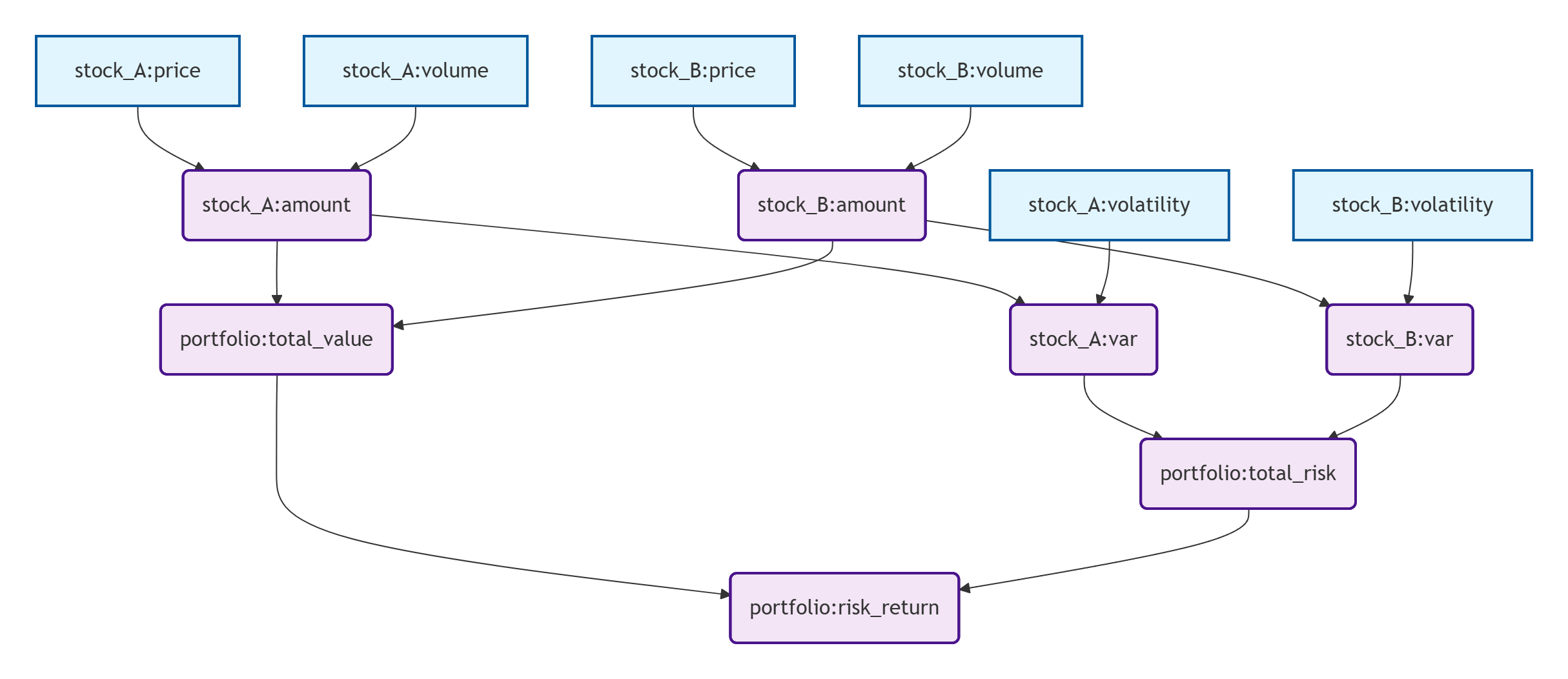
As shown above, this case begins with the basic position calculation, calculating the stock values based on the prices and quantities. Then it moves to the VaR layer, calculating the potential loss for each stock based on volatility. Portfolio risk is aggregated at the portfolio level, accounting for asset correlations to calculate the overall risk exposure. Finally, it generates a key performance indicator at the top layer, the risk-adjusted return. There are four layers of calculations in total. Each layer's calculation logic is as follows:
Layer 1: Basic Position Calculation
-
Stock A Holding Value (stock_A:amount)
-
Formula: A_Price * A_Volume
-
Dependencies: stock_A:price, stock_A:volume
-
Business meaning: Calculate the holding value of stock A in real time.
-
-
Stock B Holding Value (stock_B:amount)
-
Formula: B_Price * B_Volume
-
Dependencies: stock_B:price, stock_B:volume
-
Business meaning: Calculate the holding value of stock B in real time.
-
Layer 2: VaR Calculation
-
Stock A VaR (stock_A:var)
-
Formula: A_Amount * A_Volatility * 2.33
-
Dependencies: stock_A:amount, stock_A:volatility
-
Business meaning: Calculate the potential maximum loss of Stock A at a 95% confidence level (Z-value of 2.33), which is a classic risk measure for a single asset.
-
-
Stock B VaR (stock_B:var)
-
Formula: B_Amount * B_Volatility * 2.33
-
Dependencies: stock_B:amount, stock_B:volatility
-
Business meaning: Calculate the potential maximum loss of Stock B.
-
Layer 3: Portfolio-Level Calculation
-
Portfolio Value (portfolio:total_value)
-
Formula: A_Amount + B_Amount
-
Dependencies: stock_A:amount, stock_B:amount
-
Business meaning: Calculate the holding value of the portfolio in real time.
-
-
Portfolio Risk (portfolio:total_risk)
-
Formula: sqrt(A_VaR² + B_VaR² + 2 * 0.3 * A_VaR * B_VaR)
-
Dependencies: stock_A:var, stock_B:var
-
Business meaning: Calculate the overall risk of the portfolio's overall risk using each stock's VaR, accounting for asset correlations (assuming a correlation coefficient of 0.3). This approach is more accurate than simple addition, as it accounts for the risk diversification effect.
-
Layer 4: Integrated Performance Indicator
-
Risk-adjusted Return (portfolio:risk_return)
-
Formula: Total_Value / Total_Risk
-
Dependencies: portfolio:total_value, portfolio:total_risk
-
Business meaning: Calculate the risk-adjusted return, similar to the Sharpe ratio, which measures return per unit of risk. The higher the value, the better the portfolio's performance, as it achieves higher returns with lower risk.
-
The code is as follows:
try{dropStreamEngine("riskEngine")}catch(ex){}
// 1. Create the output table (using a key-value table, only keeping the latest state)
outputTable = keyedTable(`product`metric, 1:0, `product`metric`value, [STRING, STRING, DOUBLE])
// 2. Define dependencies (Metrics)
metrics = array(ANY, 0)
// Rule 1: Calculate the holding value of Stock A (amount = price * volume)
metricA = dict(STRING, ANY)
metricA["outputName"] = `stock_A:`amount
metricA["formula"] = <price * volume>
metricA["price"] = `stock_A:`price
metricA["volume"] = `stock_A:`volume
metrics.append!(metricA)
// Rule 2: Calculate the holding value of Stock B (amount = price * volume)
metricB = dict(STRING, ANY)
metricB["outputName"] = `stock_B:`amount
metricB["formula"] = <price * volume>
metricB["price"] = `stock_B:`price
metricB["volume"] = `stock_B:`volume
metrics.append!(metricB)
// Rule 3: Calculate the VaR of Stock A
metricAVaR = dict(STRING, ANY)
metricAVaR["outputName"] = `stock_A:`var
metricAVaR["formula"] = <2.33 * amount * volatility>
metricAVaR["amount"] = `stock_A:`amount
metricAVaR["volatility"] = `stock_A:`volatility
metrics.append!(metricAVaR)
// Rule 4: Calculate the VaR of Stock B
metricBVaR = dict(STRING, ANY)
metricBVaR["outputName"] = `stock_B:`var
metricBVaR["formula"] = <2.33 * amount * volatility>
metricBVaR["amount"] = `stock_B:`amount
metricBVaR["volatility"] = `stock_B:`volatility
metrics.append!(metricBVaR)
// Rule 5: Calculate the portfolio value
metricTotalValue = dict(STRING, ANY)
metricTotalValue["outputName"] = `portfolio:`total_value
metricTotalValue["formula"] = <A_amount + B_amount>
metricTotalValue["A_amount"] = `stock_A:`amount
metricTotalValue["B_amount"] = `stock_B:`amount
metrics.append!(metricTotalValue)
// Rule 6: Calculate the total portfolio risk based on VaR
metricTotalRisk = dict(STRING, ANY)
metricTotalRisk["outputName"] = `portfolio:`total_risk
metricTotalRisk["formula"] = <sqrt(A_var*A_var + B_var*B_var + 2 * 0.3 * A_var*B_var)>
metricTotalRisk["A_var"] = `stock_A:`var
metricTotalRisk["B_var"] = `stock_B:`var
metrics.append!(metricTotalRisk)
// Rule 7: Calculate the risk-adjusted return
metricRiskReturn = dict(STRING, ANY)
metricRiskReturn["outputName"] = `portfolio:`risk_return
metricRiskReturn["formula"] = <total_value / total_risk>
metricRiskReturn["total_value"] = `portfolio:`total_value
metricRiskReturn["total_risk"] = `portfolio:`total_risk
metrics.append!(metricRiskReturn)
// 3. Create the engine
engine = createReactiveStatelessEngine("riskEngine", metrics, outputTable)
// 4. Simulate data input
// Step1: Input basic data (price and volume)
insert into engine values("stock_A", "price", 10.5)
insert into engine values("stock_A", "volume", 1000)
insert into engine values("stock_B", "price", 20.3)
insert into engine values("stock_B", "volume", 500)
// Step2: Input risk data
insert into engine values("stock_A", "volatility", 0.15)
insert into engine values("stock_B", "volatility", 0.08)
// Step3: Update the price of Stock A and observe the chain reaction
insert into engine values("stock_A", "price", 11.2)
The output:
| product | metric | value |
|---|---|---|
| stock_A | amount | 11,200 |
| stock_A | var | 3,914.3999999999996 |
| portfolio | total_value | 21,350 |
| portfolio | total_risk | 4,831.72566853707 |
| portfolio | risk_return | 4.418711132344619 |
| stock_B | amount | 10,150 |
| stock_B | var | 1,891.96 |