Orca Declarative Stream API Application: Real-Time Monitoring of Account-Level Portfolio P&L
In modern trading systems, real-time portfolio profit and loss (P&L) calculation is a fundamental requirement for intraday risk control and portfolio management. This tutorial demonstrates how to use DolphinDB's Orca Declarative Stream API to perform a dual-stream join between tables for tick market data and snapshot data, enabling real-time monitoring of portfolio P&L.
Complete code and sample data are provided in the appendix for hands-on practice. The code has been validated on DolphinDB version 3.00.4. If you are new to the DStream API, we recommend starting with the first two chapters of the tutorial Orca Declarative Stream API Application: Real-Time Calculation of Intraday Cumulative Order-Level Capital Flow, which introduces the key components and workflow of Orca stream computing through a simple example.
1. Application Scenario
In high-speed financial markets, investors manage complex multi-asset portfolios under rapidly changing conditions, covering stocks, futures, options, forex, and cryptocurrencies. To stay competitive, they need real-time insight into portfolio P&L to manage risks, adjust strategies, and seize opportunities, as even minute- or hour-long delays can incur costs or expose them to hidden risks.
However, achieving efficient real-time monitoring across multiple assets presents several challenges:
- Massive market data streams: Handling hundreds of thousands or millions of price updates per second.
- High computational complexity: Calculating P&L requires dealing with positions, real-time prices, cost bases, potential forex conversions, and complex derivatives pricing.
- Extremely low latency requirements: Business decisions depend on near-real-time P&L updates, often within seconds or at sub-second latency.
- System scalability and maintenance challenges: Traditional batch processing or multi-component architectures often struggle with performance, latency, and scalability, while also being costly to develop and maintain.
DolphinDB's Orca, an enterprise-grade real-time computing platform, is designed to address these challenges. The Orca DStream API offers a simplified interface for defining stream processing logic, allowing users to focus on what needs to be done, rather than how to do it. Additionally, Orca's features like automated task scheduling and high availability ensure that no data is missed, improving system stability while reducing development and operational costs.
2. Implementation Solution
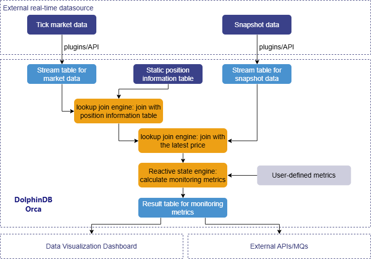
This section focuses on real-time monitoring of position P&L at the account level. The data processing is divided into two main stages:
- Stage 1-Data preprocessing: Using streaming join engines to join the market data table with the position information and snapshot data tables. This generates a comprehensive wide table, which will be used for subsequent business metric calculations.
- Stage 2-Position monitoring metrics calculation: Using the reactive state engine to calculate a set of user-defined position monitoring metrics, and you can also add personalized metrics as needed.
In this tutorial, we will simulate real-time data ingestion by replaying historical data from DolphinDB DFS tables. In practical applications, real-time data streams can be ingested into DolphinDB stream tables through MQs (e.g., Pulsar, Kafka), market data plugins (e.g., AMD, Insight), or APIs (e.g., C++, Java API).
The computed results can be accessed via external APIs or queries, or transmitted externally via MQs. This tutorial uses DolphinDB's built-in Dashboard to visualize monitoring results in real-time. For more details, refer to Section 5.3.
The overall process is shown below:
3. Data and Metrics
The tables for market data, static position information, and snapshot data used in this tutorial are all stored in DolphinDB's distributed database. We will simulate the process of continuously writing market data and snapshot data into DolphinDB stream tables through the replay function, replicating a real-world business scenario.
Sample data and import code are provided in the appendix. The sample data represents simulated data for half a trading day, in which the market data table simulates the order/fill data streams for 5 accounts holding 20 assets, the position information table simulates the position data for each asset held by these 5 accounts at market open, and the snapshot data includes L2 snapshot data for the 20 assets.
3.1 Table Schema
The specific table schema is as follows:
-
Position information table:
Table 1. Table 3-1 Position Information Table Schema Column Name Type Description AccountID SYMBOL Account ID SecurityID SYMBOL Security ID Date DATE Trade date SecurityName STRING Security name Threshold INT Threshold quantity OpenVolume INT Opening volume PreVolume INT Pre-market position PreClose DOUBLE Previous close price -
Market data table:
Table 2. Table 3-2 Market Data Table Schema Column Name Type Description AccountID SYMBOL Account ID Type INT - 1: order
- 2: fill
OrderNo INT Order number SecurityID SYMBOL Security ID Date DATE Trade date Time TIME Trade time BSFlag SYMBOL Buy/sell flag Price DOUBLE Price Volume INT Quantity TradeNo INT Trade number State SYMBOL Status: Fully filled, partially filled, canceled Mark INT Status mark:
- Fully filled: -1
- Partially filled: 1
- Canceled: 0
NetVolume INT Net buy volume CumSellVol INT Cumulative sell volume CumBuyVol INT Cumulative buy volume SellPrice DOUBLE Average sell price BuyPrice DOUBLE Average buy price ReceivedTime NANOTIMESTAMP Data receive timestamp -
Snapshot data table:
Table 3. Table 3-3 Snapshot Data Table Schema Column Name Type Description SecurityID SYMBOL Security ID Date DATE Date Time TIME Time LastPx DOUBLE Last price
3.2 Metrics Calculation Rules
This tutorial defines a series of metrics for monitoring positions. The specific meanings and code are provided below.
Note: When using user-defined functions to calculate metrics in the stream
computing engines, the @state declaration must be added before
the function definition.
CanceledVolume: Volume of canceled orders
- Formula:

TolVolumei: The initial order volume of order i.
CumVolumei: The filled order volume of order i.
- Code implementation:
@state
def calCanceledVolume(Mark, Type, Volume){
    return iif(Mark != 0, NULL, cumfirstNot(iif(Type==1, Volume, NULL)).nullFill!(0)-cumsum(iif(Mark in [-1, 1], Volume, 0)))
}PositionVolume: Real-time position volume
- Formula:

- Code implementation:
@state
def calPositionVolume(Type, PreVolume, CumBuyVol, CumSellVol){
    positionVolume = iif(Type==2, PreVolume+CumBuyVol-CumSellVol, ffill(PreVolume+CumBuyVol-CumSellVol))
    return iif(isNull(positionVolume), PreVolume, positionVolume)
}ThresholdDeviation: Threshold deviation
- Formula:

- Code implementation:
@state
def calThresholdDeviation(Type, PreVolume, CumBuyVol, CumSellVol, Threshold){
    thresholdDeviation = iif(Threshold>0 and calPositionVolume(Type, PreVolume, CumBuyVol, CumSellVol)>0, (calPositionVolume(Type, PreVolume, CumBuyVol, CumSellVol)-Threshold)\Threshold, 0)
    return round(thresholdDeviation, 6)
}PositionDeviation: Position deviation
- Formula:

- Code implementation:
@state
def calPositionDeviation(Type, OpenVolume, PreVolume, CumBuyVol, CumSellVol){
	positionDeviation = iif(OpenVolume>0 and calPositionVolume(Type, PreVolume, CumBuyVol, CumSellVol)>0, calPositionVolume(Type, PreVolume, CumBuyVol, CumSellVol)\OpenVolume-1, 1)
	return round(positionDeviation, 6)
}BuyVolume: Buy volume for the day
- Formula:

- Code implementation:
@state
def calBuyVolume(Type, CumBuyVol){
    buyVolume = iif(Type==2, CumBuyVol, ffill(CumBuyVol))
    return iif(isNull(buyVolume), 0, buyVolume)
}BuyPrice: Average buy price for the day
- Formula:

n: The number of buy orders executed from the start of the day to the current time.
Pricei: Price of buy order i.
Volumei: Volume of buy order i.
- Code implementation:
@state
def calBuyPrice(Type, BSFlag, CumBuyVol, BuyPrice){
    buyPrice = cumsum(iif(isNull(prev(deltas(ffill(CumBuyVol)))) and CumBuyVol!=NULL, BuyPrice*CumBuyVol, ffill(BuyPrice)*deltas(ffill(CumBuyVol))))\ffill(CumBuyVol)
    return round(iif(isNull(buyPrice), 0, buyPrice), 6)
}SellVolume: Sell volume for the day
- Formula:

- Code implementation:
@state
def calSellVolume(Type, CumSellVol){
    sellVolume = iif(Type==2, CumSellVol, ffill(CumSellVol))
    return iif(isNull(sellVolume), 0, sellVolume)
}SellPrice: Average sell price for the day
- Formula:

m: The number of sell orders executed from the start of the day to the current time.
Pricej: Price of sell order j.
Volumej: Volume of sell order j.
- Code implementation:
@state
def calSellPrice(Type, BSFlag, CumSellVol, SellPrice){
    sellPrice = cumsum(iif(isNull(prev(deltas(ffill(CumSellVol)))) and CumSellVol!=NULL, SellPrice*CumSellVol, ffill(SellPrice)*deltas(ffill(CumSellVol))))\ffill(CumSellVol)
    return round(iif(isNull(sellPrice), 0, sellPrice), 6)
}NetBuyVolume: Net buy volume for the day
- Formula:

- Code implementation:
@state
def calNetBuyVolume(NetVolume){
    netBuyVolum = ffill(NetVolume)
    return iif(isNull(netBuyVolum), 0, netBuyVolum)
}FreezeVolume: Frozen position volume
- Formula:

CanceledVolumesi: The cancellation volume in sell order i.
- Code implementation:
@state
def calFreezeVolume(VOLUME, BSFlag, Mark, Type){
	return cumsum(iif(BSFlag=="B", 0, iif(Mark==0, -calCanceledVolume(Mark, Type, VOLUME), iif(Mark in [1, -1], -VOLUME, VOLUME))))
}AvailableVolume: Available position volume
- Formula:

- Code implementation:
@state
def calAvailableVolume(Type, PreVolume, CumBuyVol, CumSellVol, VOLUME, BSFlag, Mark){
	availableVolume = PreVolume-calSellVolume(Type, CumSellVol)-calFreezeVolume(VOLUME, BSFlag, Mark, Type)
	return availableVolume
}AvailableVolumeRatio: Available position ratio
- Formula:

- Code implementation:
@state
def calAvailableVolumeRatio(Type, PreVolume, CumBuyVol, CumSellVol, VOLUME, BSFlag, Mark){
	availableVolumeRatio = calAvailableVolume(Type, PreVolume, CumBuyVol, CumSellVol, VOLUME, BSFlag, Mark)\PreVolume
	return round(iif(isNull(availableVolumeRatio), 0, availableVolumeRatio), 6)
}Profit: P&L for the day
- Formula:

- Code implementation:
@state
def calProfit(Type, PreVolume, BSFlag, SellPrice, BuyPrice, CumSellVol, CumBuyVol, LastPx, PreClose){
    profit = (PreVolume-calSellVolume(Type, CumSellVol))*(LastPx-PreClose)+calSellVolume(Type, CumSellVol)*(calSellPrice(Type, BSFlag, CumSellVol, SellPrice)-PreClose)+calBuyVolume(Type, CumBuyVol)*(LastPx-calBuyPrice(Type, BSFlag, CumBuyVol, BuyPrice))
    return round(profit, 6)
}
4. Code Implementation for Monitoring Position
This chapter first introduces the code for building real-time position monitoring metric calculation tasks using the DStream API, followed by the data replay code to simulate real-time calculation tasks. The full code is provided in the appendix.
4.1 Construct Stream Graph
This section will guide you through the step-by-step process of constructing a stream graph to implement real-time calculation of position monitoring metrics.
(1) Create Data Catalog and Stream Graph
First, create a data catalog named positionMonitorDemo, and then create a stream graph positionMonitor under the positionMonitorDemo catalog. The code is as follows:
// Create a data catalog
if (!existsCatalog("positionMonitorDemo")) {
	createCatalog("positionMonitorDemo")
}
go
// Create a stream graph
use catalog positionMonitorDemo
try { dropStreamGraph("positionMonitor") } catch (ex) {}
positionMonitorGraph = createStreamGraph("positionMonitor")
(2) Create Stream Tables
The next step is to define the data sources within the stream graph. The code is as follows:
// Market data table
colNameMarketData = `AccountID`Type`OrderNo`SecurityID`Date`Time`BSFlag`Price`Volume`TradeNo`State`Mark`NetVolume`CumSellVol`CumBuyVol`SellPrice`BuyPrice`ReceivedTime
colTypeMarketData = `SYMBOL`INT`INT`SYMBOL`DATE`TIME`SYMBOL`DOUBLE`INT`INT`SYMBOL`INT`INT`INT`INT`DOUBLE`DOUBLE`NANOTIMESTAMP
MarketDataStream = positionMonitorGraph.source("MarketDataStream", colNameMarketData, colTypeMarketData).parallelize("AccountID", 2)
// Position monitoring information table
colNamePositionInfo = `AccountID`SecurityID`Date`SecurityName`Threshold`OpenVolume`PreVolume`PreClose
colTypePositionInfo = `SYMBOL`STRING`DATE`STRING`INT`INT`INT`DOUBLE
PositionInfo = positionMonitorGraph.source("PositionInfo", colNamePositionInfo, colTypePositionInfo)
// Snapshot data table
colNameSnapshot = `SecurityID`Date`Time`LastPx
colTypeSnapshot = `SYMBOL`DATE`TIME`DOUBLE
SnapshotStream = positionMonitorGraph.source("SnapshotStream", colNameSnapshot, colTypeSnapshot)
The StreamGraph::source method is used to define persistent,
shared stream data tables as data sources. Given the large volume of market
data, the DStream::parallelize method is used to
hash-partition the data by AccountID, generating parallel branches, which
improves data processing efficiency.
(3) Join Market Data with Position Information
To calculate position monitoring metrics, join the market data table with the position information table to retrieve the historical position data. The code is as follows:
// Join with position information table
marketJoinPositionInfo = MarketDataStream.lookupJoinEngine(
    rightStream = PositionInfo,
    metrics = [
        <Type>, <OrderNo>, <Date>, <Time>, <BSFlag>, <Price>,
        <Volume>, <TradeNo>, <State>, <Mark>, <NetVolume>, <CumSellVol>,
        <CumBuyVol>, <SellPrice>, <BuyPrice>, <ReceivedTime>, <SecurityName>,
        <Threshold>, <OpenVolume>, <PreVolume>, <PreClose>
    	],
    matchingColumn = `AccountID`SecurityID,
    rightTimeColumn = `Date
    )
Use the DStream::lookupJoinEngine method to create a join
engine in the stream graph. Here, the matchingColumn specifies the
columns for joining the left and right tables, and the
rightTimeColumn specifies the time column for the right
table.
(4) Join with Snapshot Data
To calculate real-time P&L, price information should be retrieved. The following code shows how to join the market data with snapshot data:
// Join each fill with the corresponding snapshot to get the latest market price
marketJoinSnapshot = marketJoinPositionInfo.lookupJoinEngine(
	rightStream = SnapshotStream,
	metrics = [
		<AccountID>, <Type>, <OrderNo>, <Date>, <Time>, <BSFlag>, <Price>,
        <Volume>, <TradeNo>, <State>, <Mark>, <NetVolume>, <CumSellVol>,
        <CumBuyVol>, <SellPrice>, <BuyPrice>, <ReceivedTime>, <SecurityName>,
        <Threshold>, <OpenVolume>, <PreVolume>, <PreClose>, <LastPx>
		],
	matchingColumn = `SecurityID,
	rightTimeColumn = `Date
	)
Using DStream::lookupJoinEngine again can create an engine
to join the output data from the reactive state engine with snapshot data.
When market data is updated, the new records will fetch the corresponding
latest price from the snapshot data via the join engine.
(5) Calculate Metrics
After the streaming data is joined, the following code calculates the position monitoring metrics:
// Real-time calculation of monitoring metrics
metrics = [<ReceivedTime>, <Date>, <Time>, <SecurityName>
	, <calPositionVolume(Type, PreVolume, CumBuyVol, CumSellVol) as `PositionVolume>
	, <Threshold>
	, <calThresholdDeviation(Type, PreVolume, CumBuyVol, CumSellVol, Threshold) as `ThresholdDeviation>
	, <OpenVolume>
	, <calPositionDeviation(Type, OpenVolume, PreVolume, CumBuyVol, CumSellVol) as `PositionDeviation>
	, <PreClose>, < PreVolume>
	, <calBuyVolume(Type, CumBuyVol) as `BuyVolume>
	, <calBuyPrice(Type, BSFlag, CumBuyVol, BuyPrice) as `BuyPrice>
	, <calSellVolume(Type, CumSellVol) as `SellVolume>
	, <calSellPrice(Type, BSFlag, CumSellVol, SellPrice) as `SellPrice>
	, <calNetBuyVolume(NetVolume) as `NetBuyVolume>
	, <calAvailableVolume(Type, PreVolume, CumBuyVol, CumSellVol, Volume, BSFlag, Mark) as `AvailableVolume>
	, <calAvailableVolumeRatio(Type, PreVolume, CumBuyVol, CumSellVol, Volume, BSFlag, Mark) as `AvailableVolumeRatio>
	, <calFreezeVolume(Volume, BSFlag, Mark, Type) as `FreezeVolume>
	, <LastPx>
	, <calProfit(Type, PreVolume, BSFlag, SellPrice, BuyPrice, CumSellVol, CumBuyVol, LastPx, PreClose) as `Profit>
	, <now(true) as UpdateTime>
    ]
positionMonitor = marketJoinSnapshot.reactiveStateEngine(
	metrics=metrics,
	keyColumn=`AccountID`SecurityID,
	keepOrder=true)
	.sync()
	.sink("PositionMonitorStream")
In the reactive state engine, the previously defined functions are called to
calculate metrics by grouping based on the account ID and security ID. This
engine triggers an output each time it receives an input, and applies
incremental computation optimizations to common state functions (moving
functions, cumulative functions, order-sensitive functions, topN functions,
etc.), greatly improving computation efficiency.
DStream::sync is used to merge parallel computation
paths and must be called with DStream::parallelize. After
all calculations are completed, use DStream::sink to output
streaming data to a persistent shared table.
(6) Submit the Stream Graph
Finally, use the StreamGraph::submit method to submit the
stream graph.
Note: The stream graph will not start without calling
submit.
The code is as follows:
// Submit the stream graph
positionMonitorGraph.submit()
4.2 Data Replay
Since it stores static data, the positionInfo table can be batch-inserted before
the market opens each day using the appendOrcaStreamTable
method.
To simulate the real-time transmission of market and snapshot data, this tutorial
uses the useOrcaStreamTable function, which locates and
retrieves the stream table by its name at the corresponding node, and then
passes this table as the first parameter to the user-defined function for
execution. The code is as follows:
// Write position information before market opens
positionInfo = select * from loadTable("dfs://positionMonitorData", "positionInfo")
appendOrcaStreamTable("PositionInfo", positionInfo)
// Data replay to simulate real-time data writing
// Replay market data
useOrcaStreamTable("MarketDataStream", def (table) {
    submitJob("replayOrderTrade", "replayOrderTrade", def (table) {
        ds1 = replayDS(sqlObj=<select * from loadTable("dfs://positionMonitorData", "marketData") where Date=2023.02.01>, dateColumn=`Date, timeColumn=`Time, timeRepartitionSchema=cutPoints(09:30:00.000..15:00:00.000, 50))
        replay(inputTables=ds1, outputTables=table, dateColumn=`Date, timeColumn=`Time, replayRate=1, absoluteRate=false, preciseRate=true)
    }, table)
})
// Replay snapshot data
useOrcaStreamTable("SnapshotStream", def (table) {
    submitJob("replaySnapshot", "replaySnapshot", def (table) {
        ds2 = replayDS(sqlObj=<select * from loadTable("dfs://positionMonitorData", "snapshot") where Date=2023.02.01>, dateColumn=`Date, timeColumn=`Time, timeRepartitionSchema=cutPoints(09:30:00.000..15:00:00.000, 50))
        replay(inputTables=ds2, outputTables=table, dateColumn=`Date, timeColumn=`Time, replayRate=1, absoluteRate=false, preciseRate=true)
    }, table)
})
This section simulates the real-time snapshot data input through data replay. The
replayDS function replays the data in sequence through
dividing SQL queries into multiple time-based data sources as inputs for the
replay function, where the timeRepartitionSchema
parameter partitions data sources, and the cutPoints function
divides the trading day into 50 buckets. With replayRate=1 and
absoluteRate=false, the data is replayed at the same speed it was
originally recorded. Finally, the submitJob function submits
the replay task to the node where the Orca stream table is located.
5. Result Display
This chapter demonstrates how to view the stream graph's running status and calculation results after constructing the stream graph and performing data replay.
5.1 View Stream Graph Status
After creating the stream graph, you can check its running status through the Web Interface or Orca APIs.
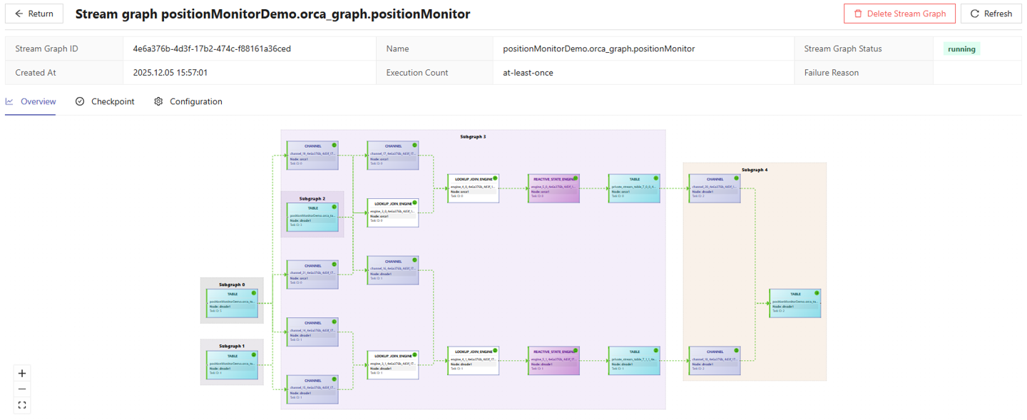
(1) View Status From Web Interface
After submitting the stream graph, you can view its structure in the
Stream Graph interface. When using the
DStream::parallelize method with the parallelism
set to 2, the stream graph appears as shown in the figure below:
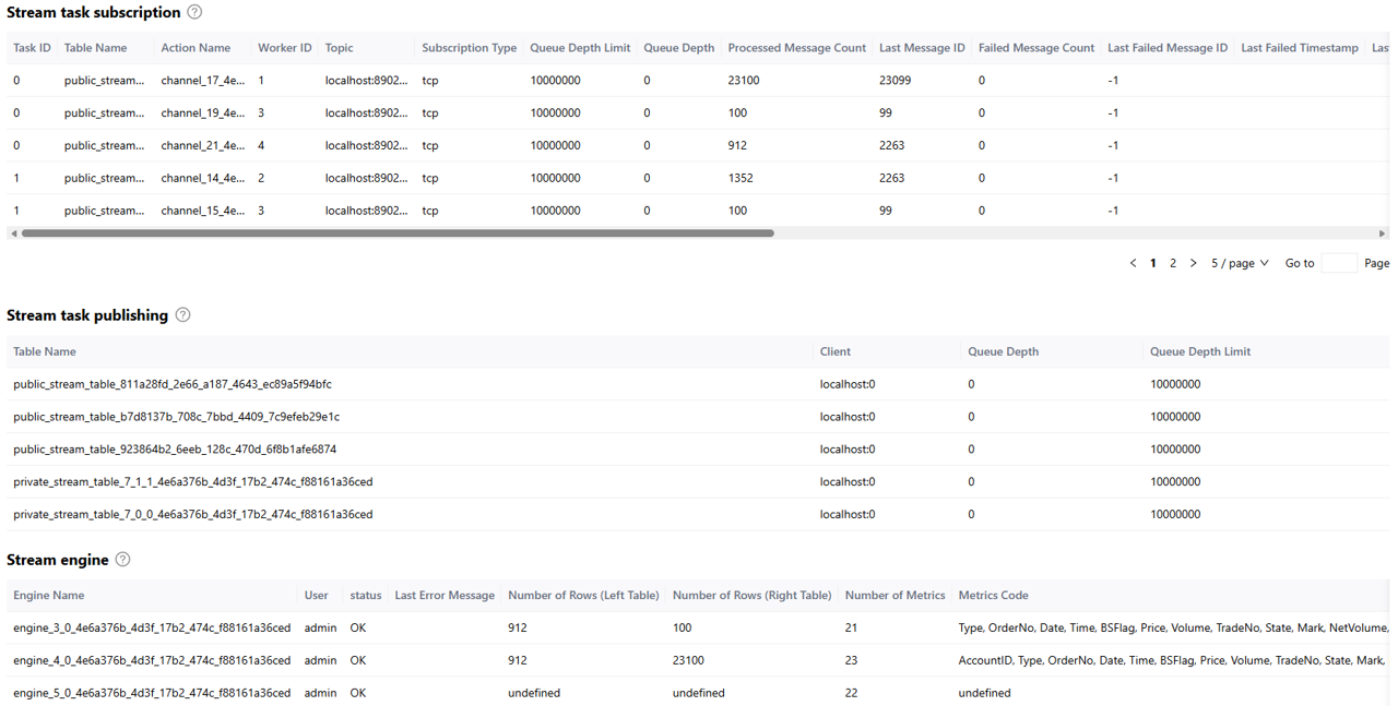
By referring to the tables below, such as Stream task subscription, Stream task publishing, and Stream engine, you can monitor the real-time status of the workers on subscribers, connection status between the local publisher and its subscribers, as well as the status of engines and tables, as shown in the figure below:
(2) View Status via Functions
Orca provides a rich set of maintenance functions for stream graph monitoring. The Web Interface outputs tables containing meta information returned from these functions.
getStreamGraphInfo: Get the structure, scheduling, and meta
information of the stream graph.
getStreamGraphInfo("positionMonitorDemo.orca_graph.positionMonitor")getOrcaStreamTableMeta: Get meta information of a specific
stream table within the stream graph.
getOrcaStreamTableMeta('positionMonitorDemo.orca_table.MarketDataStream')getOrcaStreamEngineMeta: Get meta information of all
streaming engines within the stream graph.
getOrcaStreamEngineMeta("positionMonitorDemo.orca_graph.positionMonitor")For more information on Orca maintenance functions, refer to Orca API Reference。
5.2 View Calculation Results
You can query the calculation results of the position monitoring metrics using the following SQL statement:
result = select * from positionMonitorDemo.orca_table.PositionMonitorStreamHere, PositionMonitorStream is the stream table previously defined to store the calculation results. When querying object within the stream graph, specify its fully qualified name. The query results are shown below:

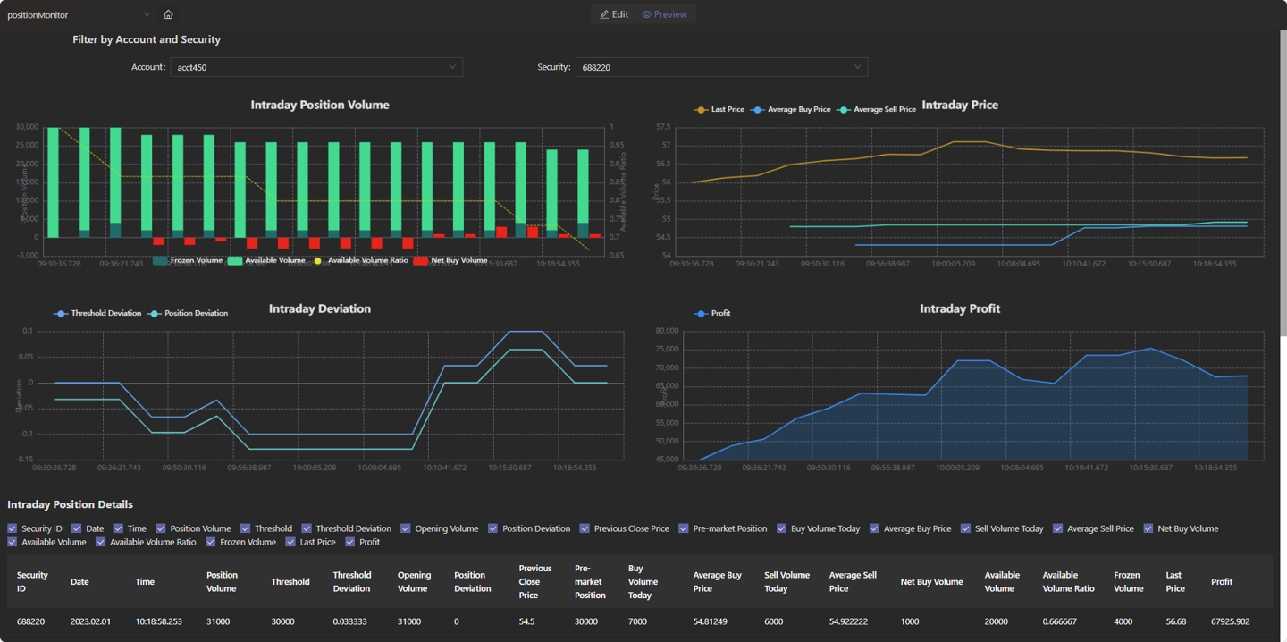
5.3 Result Visualization
By editing the Dashboard of Web Interface, you can visualize the calculation results, as shown in the figure below. The JSON configuration file for this dashboard is provided in the appendix.
6. Performance Test
In this tutorial, we test the calculation latency for completing 12 monitoring metrics per market data record by replaying large volumes of historical data. The latency refers to the time difference between calculation completion (UpdateTime) and data arrival (ReceiveTime). We calculate the average and 99th percentile of the latency for all records, where the 99th percentile represents the value below which the latency for 99% of the records falls.
Additional tests evaluate the performance under varying concurrency and replay speeds. Different replay speeds correspond to different data volumes. The 5x speed replay simulates a high-load scenario, where the order/fill processing throughput (TPS) reaches up to 50,000 per second.
6.1 Test Data Volume
- Simulated market data streams
- 10,000 records per second
- 3,000 securities
- 800 accounts (each with over 2,300 securities)
- A total of 72,026,955 records (from 09:30 to 11:30, half a trading day)
- Simulated static position information
- Simulated data
- Each record represents the position of one security held by one of the 800 accounts on that day
- Real snapshot data
- Level-2 stock market snapshot with a frequency of 3 seconds
6.2 Test Results
Latency unit: microseconds
| Concurrency | Replay Speed | Market Data Flow (TPS) | Total Latency (Average/99th Percentile) |
|---|---|---|---|
| 8 | 1X | 1w | 743 / 1622 |
| 16 | 1X | 1w | 697 / 1391 |
| 8 | 5X | 5w | 1045 / 8928 |
| 16 | 5X | 5w | 877 / 4155 |
- At concurrency level 8 with a data flow of 10,000 TPS, the average end-to-end latency is 743 microseconds.
- Similarly, even at 50,000 TPS with the same concurrency, latency remains around 1 millisecond.
- Increasing concurrency further reduces computation latency. Specifically, under high load, increasing from 8 to 16 concurrency halves the 99th percentile latency by leveraging additional computational power for better peak performance.
6.3 Test Environment
This test uses the standalone mode of the DolphinDB server. Specific environment configuration is shown in the table below:
| Environment | Model/Configuration/Software Name/Version |
|---|---|
| DolphinDB | 3.00.4 2025.09.09 LINUX_JIT x86_64 |
|
Physical Server x 1 |
Operating System: CentOS Linux 7 (Core) |
| Kernel: 3.10.0-1160.el7.x86_64 | |
| CPU: Intel(R) Xeon(R) Gold 5220R CPU @ 2.20GHz | |
| License Limit: 8 cores, 256 GB RAM | |
| Configured Maximum available memory for test node: 256 GB |
7. Summary and Outlook
The Orca declarative stream API simplifies stream computing through concise programming with DolphinDB. Based on Orca, this tutorial provides a low-latency solution for real-time metrics monitoring, serving as a reference for developers to develop high-performance stream computing for business scenarios, thereby improving development efficiency.
In the future, Orca will introduce the following core features and optimizations. With the low-latency technology outlined below, the response speed of monitoring portfolio in this tutorial will be further enhanced.
- Low-latency engine: Supports ultra-low latency at the 10-microsecond level.
- Streaming SQL engine: Integrates low-latency streaming SQL computation.
- High availability: Supports full-memory, ultra-low-latency high availability.
- JIT compilation: Supports operator fusion and just-in-time compilation for streaming engines.
- Development and debugging: Offers more user-friendly stream computing task development and debugging tools.
Orca aims to provide a comprehensive technical foundation for financial institutions to build a next-generation internal unified platform, enhancing the institutions' response time from T+1 to T+0, or even down to the microsecond level.
Appendix
-
Example code for calculating position monitoring: PositionMonitor.dos
-
Example code for creating database & tables and importing example data: importData.dos
-
Example data: SampleData.zip
-
Dashboad configuration file: dashboard.positionMonitor.json