Orca Declarative Stream API Application: Real-Time Calculation of Intraday Cumulative Order-Level Capital Flow
Stream computing has always been one of the core functionalities of DolphinDB products. With its feature-rich stream computing engine and high-performance built-in operators, DolphinDB has helped numerous clients achieve high-performance real-time computing production deployments in scenarios such as factor calculation and trading monitoring. As the industry deepens its use of stream computing, enterprises have raised higher requirements for streaming data products. For this reason, DolphinDB's stream computing functionality module continues to evolve, and in version 3.00.3, it released the enterprise-level real-time computing platform Orca. Based on the original stream computing products, Orca provides users with more concise programming APIs, clearer task management, more intelligent automatic scheduling, and more reliable high-availability computing support. For a more detailed introduction to Orca, please refer to Orca.
This tutorial focuses on introducing the Declarative Stream API (DStream API) that Orca provides for stream computing jobs. The DStream API offers users a more concise interface design with higher abstraction levels. With declarative programming paradigm at its core, it allows users to define stream data processing logic by describing "what to do" rather than "how to do it", thereby lowering the development threshold for stream processing applications. This enables developers to focus on more macro-level business logic and requirements without concerning themselves with implementation details, while also reducing code maintenance and modification costs.
This tutorial will introduce how to build stream computing jobs using DStream API through two specific financial scenario cases. First, through a simple introductory case, we'll introduce the key components and development process of Orca stream computing jobs. Then we'll further demonstrate how to use DStream API to implement more complex business scenarios—real-time daily cumulative order-by-order capital flow calculation.
All scripts in this article are developed and run on compute nodes of DolphinDB cluster compute groups deployed on Linux version 3.00.3. Users can also quickly try DStream API in standalone mode.
1. DolphinDB Stream Computing Programming Interfaces
Before entering the DStream API cases in subsequent chapters, we will first review the several abstraction levels of DolphinDB stream computing programming in this chapter. This chapter is mainly for users who have used DolphinDB stream computing frameworks in versions prior to 3.00.3, intended to briefly introduce the relationship between DStream API and previously existing interfaces. Readers may also skip this chapter and directly follow subsequent chapters to learn DStream API usage.
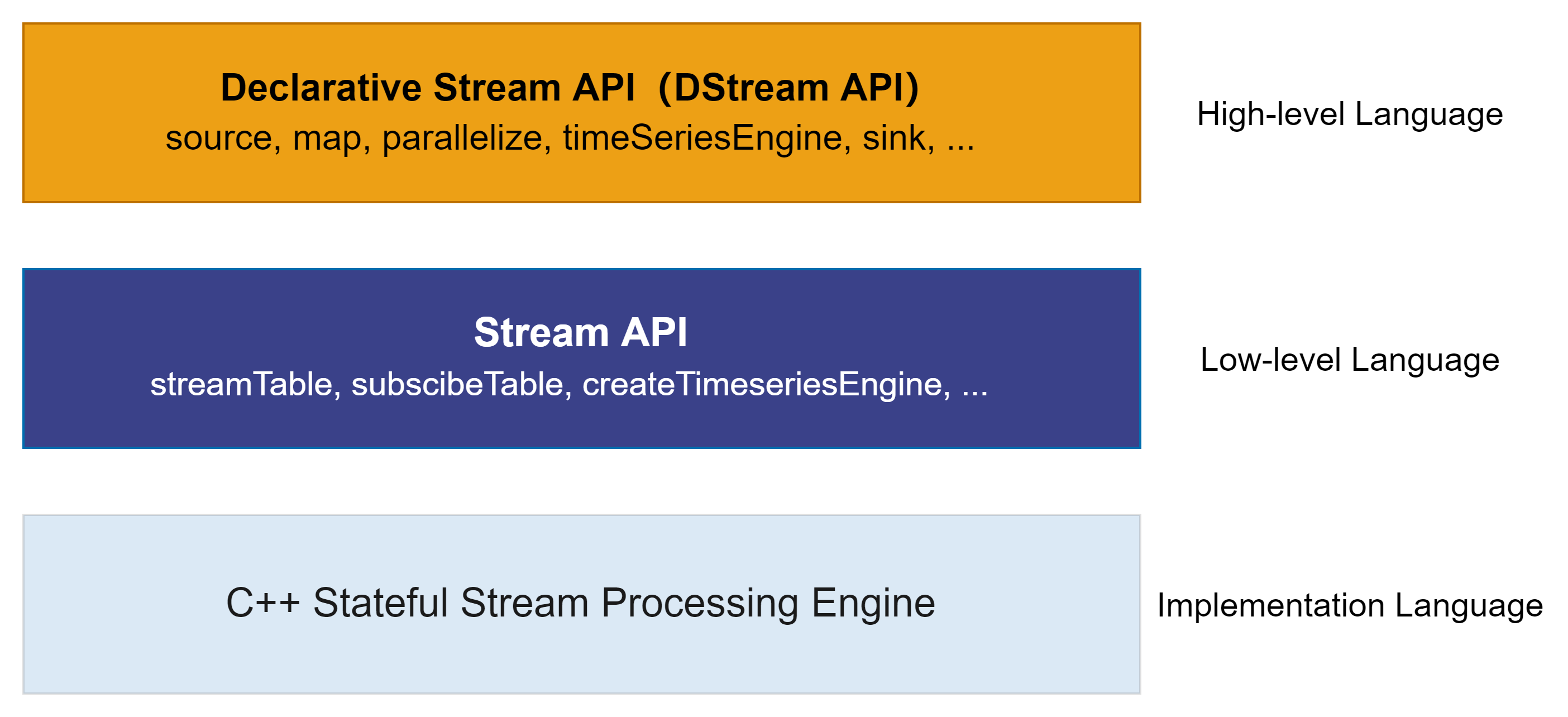
DolphinDB's underlying implementation language is C++, which ensures its high performance in real-time computing scenarios. At the upper level, DolphinDB exposes well-abstracted programming interfaces to users through its scripting language (DLang), allowing users to use DolphinDB's stream computing framework through these interfaces.
Prior to version 3.00.3, DolphinDB stream computing only provided functional
programming interfaces—Stream API. Users created stream tables, subscriptions,
engines, etc., through function calls (such as streamTable,
subscribeTable, createReactiveStateEngine,
etc.), and completed stream computing job construction by connecting stream tables,
subscriptions, engines, and other modules in a building-block manner.
Starting from version 3.00.3, DolphinDB stream computing provides further abstracted programming interfaces—DStream API. DStream API shields complex logic such as underlying parallel scheduling, subscription relationships, and resource cleanup. Users can more concisely define processing logic through chain programming. The underlying system will convert user-defined DStream API into DolphinDB function calls and automatically package them as stream tasks for distribution to various nodes for execution. See DStream API interface list: Orca API Reference.
The following is sample DStream API code, which we will break down and introduce in the next chapter.
g = createStreamGraph("quickStart")

g.source("trade",`securityID`tradeTime`tradePrice`tradeQty`tradeAmount`buyNo`sellNo, [SYMBOL,TIMESTAMP,DOUBLE,INT,DOUBLE,LONG,LONG])
.map(msg -> select * from msg where tradePrice!=0)
.reactiveStateEngine(
        metrics = [<tradeTime>, <tmsum(tradeTime, iif(buyNo>sellNo, tradeQty, 0), 5m)\tmsum(tradeTime, tradeQty, 5m) as factor>],
        keyColumn = ["SecurityID"])
.sink("resultTable")

g.submit()
2. Orca Stream Computing Job Code Analysis
This chapter introduces the fundamental components of the code for an Orca stream processing job, using an introductory example to help new users quickly get started with the DStream API.
2.1 Core Components
An Orca stream job typically consists of the following five components:
- Create a stream graph in a specified catalog
- Specify or create a data source
- Define the data transformation logic
- Specify the output table for computation results
- Submit the stream graph
Once the stream graph is submitted, the job is formally launched in the background. By default, data consumption begins from the earliest available record in the source stream. As the source stream continuously receives new records, the transformation will continue until the stream graph is destroyed.
The following example demonstrates how to use the DStream API in Orca to perform real-time computation of the active trading volume ratio over the past 5 minutes.
2.2 Quick Start: 5-Minute Active Trading Volume Ratio
This example utilizes tick-by-tick trading data streams as input, implementing real-time response to individual records, calculating and outputting the active trading volume ratio over the preceding 5-minute interval.
Factor Computation Logic
Active trading ratio represents the proportion of active trading volume relative
to total trading volume. The formula is as follows: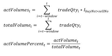
Where:
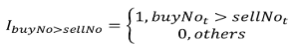
- actVolumeₜ denotes active trading volume within the interval
[t-window, t]. Indicator function IbuyNo>selNo is defined as:
- totalVolumeₜ represents total trading volume within the interval [t-window, t].
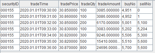
Sample Input Data
The subsequent implementation progressively constructs the stream computing job using DStream API. The full script is provided in the appendix.
(1) Create a stream graph in a catalog
use catalog tutorial
g = createStreamGraph("quickStart")- DolphinDB implements catalogs for unified organization of database objects, including distributed table. Orca extends catalog application scope to encompass stream graphs, stream tables, and stream engines within the catalog structure, enabling unified access to diverse elements.
- A stream processing workflow constructed using DStream API is abstracted as a Directed Acyclic Graph (DAG), known as a stream graph. Each node represents a stream table or stream engine, and each edge defines a data flow relationship between nodes.
- The
createStreamGraphfunction initializes a new stream graph. Through method chaining, this stream graph can be enhanced by appending data source nodes, stream computing engine nodes, etc., from this initialization point to complete stream computing job definition. - A stream graph is uniquely identified by
<catalog>.orca_graph.<name>. It is recommended that each user or project utilize distinct catalogs to prevent stream graph naming conflicts between users and avoid conflicts among stream tables and engines within stream graphs. - The function
createStreamGraphreturns a StreamGraph object.
Ensure that the catalog tutorial exists before use. If not, you
can create it using:
createCatalog("tutorial")(2) Specify or create the data source
sourceStream = g.source(
    "trade_original",
    `securityID`tradeTime`tradePrice`tradeQty`tradeAmount`buyNo`sellNo,
    [SYMBOL,TIMESTAMP,DOUBLE,INT,DOUBLE,LONG,LONG]
)- A data source (source node) is essentially a stream table that holds the
incoming data to be processed. In this example, we use
StreamGraph::sourceto create a persistent shared stream table. Subsequently, we will simulate data ingestion into this table to trigger the factor computation. - Alternatively, the method
StreamGraph::sourceByNamecan be used to reference an existing stream table in the system. For example:sourceByName(marketData.orca_table.trade) - The
sourcemethod returns aDStreamobject.
(3) Define the data transformation logic
transformedStream = sourceStream.map(msg -> select * from msg where tradePrice != 0)
    .reactiveStateEngine(
        metrics = [
            <tradeTime>,
            <tmsum(tradeTime, iif(buyNo > sellNo, tradeQty, 0), 5m)\tmsum(tradeTime, tradeQty, 5m) as factor>
        ],
        keyColumn = ["SecurityID"]
)DStreamobjects represent data streams. Stream transformations can be performed through theDStream::mapmethod and various engine methods (DStream::reactiveStateEngine,DStream::timeSeriesEngine, etc.). Each transformation returns a newDStreamobject.- The
DStream::mapmethod primarily defines stateless operations, such as filtering records with non-zero trade prices in this case. - Various engine methods accommodate stateful streaming computations across
different scenarios. Users require only basic engine parameter
configuration, with streaming implementation and state management handled by
underlying engine architectures. For instance,
reactiveStateEnginesupports record-by-record response computation in this example where computation results depend on historical data. Subsequently, we will utilizedailyTimeSeriesEnginefor window aggregation and downsampling. - The metrics within
DStream::reactiveStateEnginedefines factor computation logic.tradeTimespecifies output of the input tradeTime column alongside computation results, whiletmsum(tradeTime, iif(buyNo>sellNo, tradeQty, 0), 5m)\tmsum(tradeTime, tradeQty, 5m)specifies output of the calculated active trading volume ratio as a computation result column. tmsumis a built-in DolphinDB function for sliding window aggregation. It is optimized for incremental computation and can be used in both batch (SQL engine) and streaming (e.g., reactive state engine) contexts.
(4) Specify the output table
transformedStream.sink("resultTable")The DStream::sink method specifies the target table for
transformed data stream output, supporting both persistent shared stream tables
and DFS library tables. In this example, results are written to a persistent
shared stream table named resultTable. Calling sink also
creates the table and allows for configuration such as cacheSize.
(5) Submit the stream graph
g.submit()- The
g.submit()statement submits the defined stream graph, formally launching the stream computing job. - Upon submission, the logical stream graph is converted into a physical stream graph. The conversion process encompasses private stream table addition, optimization, and parallelism partitioning. These implementation details are fully abstracted in the declarative API.
- Once submitted, the stream graph can be monitored via the Web UI. Clicking
on the stream graph name reveals detailed information, including a
visualized physical graph and subscription thread status.
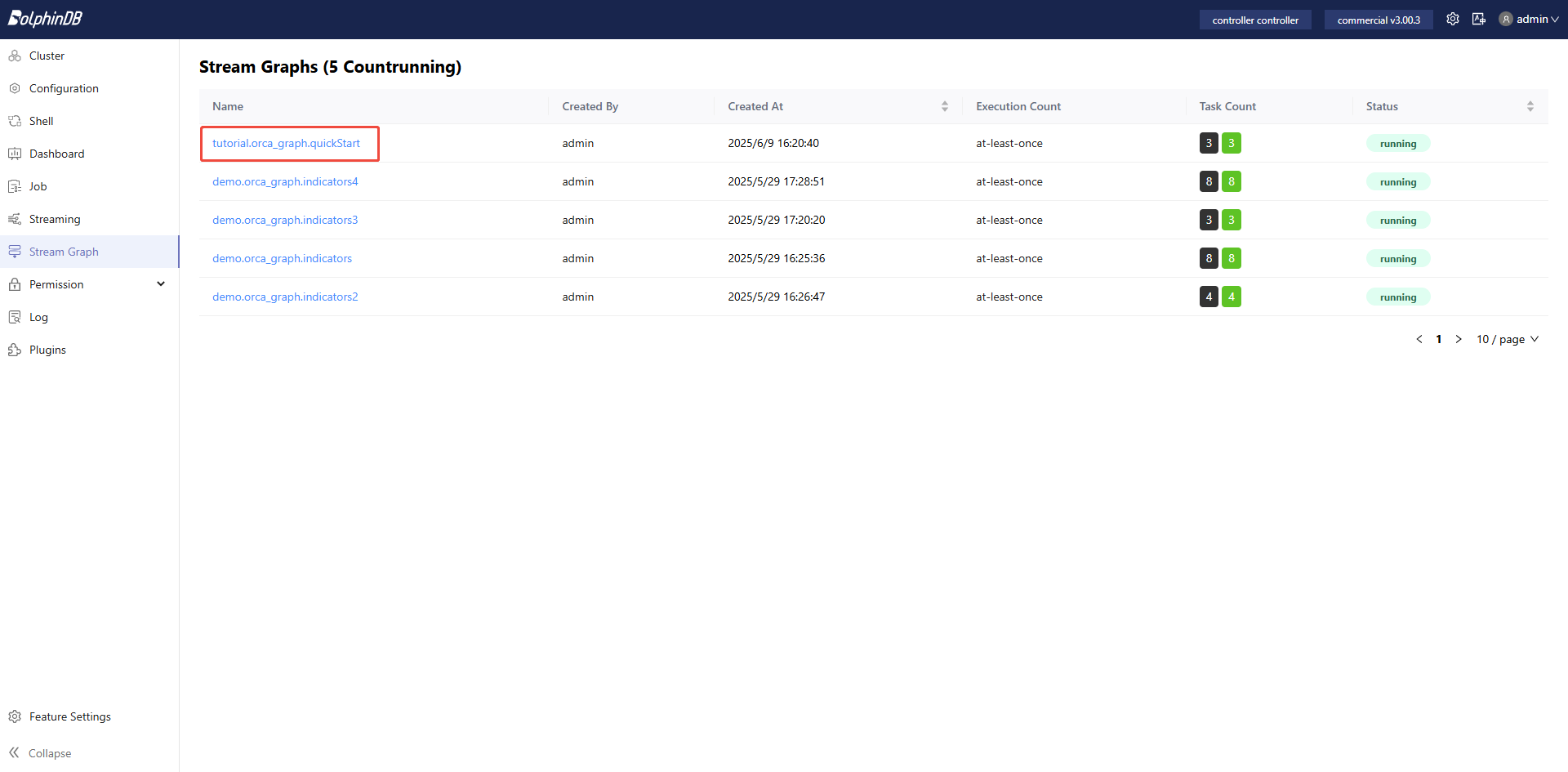
Figure 2. Figure 2-1 Stream Graph List - Tasks within the physical stream graph are automatically split and
dispatched across different nodes for parallel execution.
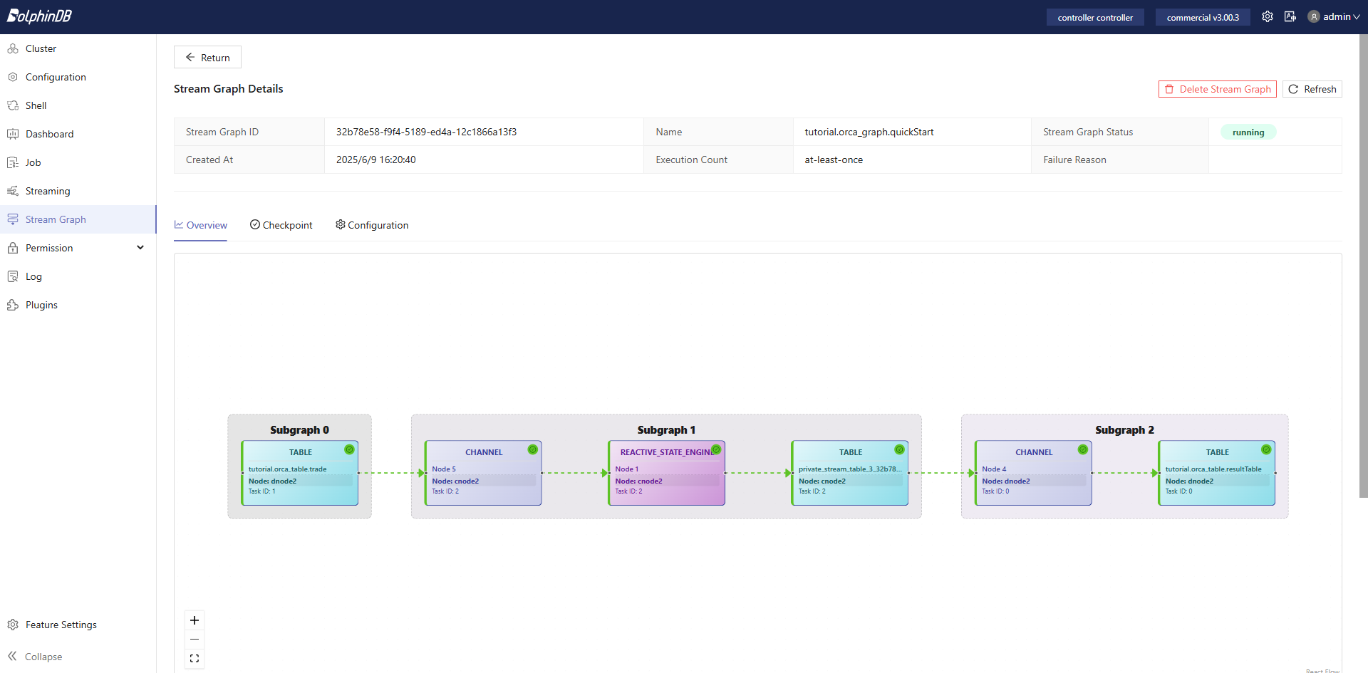
Figure 3. Figure 2-2 Physical Stream Graph
Simulate Data and View Output
The following code simulates a few records and writes them to the
demo.orca_table.trade stream table, triggering the
computation defined in the submitted stream graph.
securityID = take(`000000, 7)
tradeTime = 2020.01.01T09:30:00.000 + 60000 * 0..6
tradePrice = [30.85, 30.86, 30.85, 30.83, 30.82, 30.82, 30.87]
tradeQty = [100, 100, 200, 100, 300, 500, 800]
tradeAmount = [3085, 3086, 6170, 3083, 9246, 15410, 24696]
buyNo = [4951, 4952, 5001, 5202, 5506, 5510, 5700]
sellNo = [0, 1, 5100, 5204, 5300, 5600, 5600]
data = table(securityID, tradeTime, tradePrice, tradeQty, tradeAmount, buyNo, sellNo)
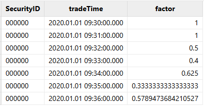
appendOrcaStreamTable("tutorial.orca_table.trade", data)Results can be queried through SQL statements:
select * from tutorial.orca_table.resultTableThe calculation results are as follows:
We have completed a full example of factor computation using Orca DStream API. In the next section, we will explore a more complex business scenario to further demonstrate the capabilities of DStream API.
3. Application Case: Real-time Daily Cumulative Order-by-Order Capital Flow
This chapter presents an Orca application within production business scenarios, utilizing DStream API for daily cumulative order-by-order capital flow computation. Compared to the foundational example in Chapter 2, this scenario implements more complex computation logic and utilizes real data replay as the data source. This scenario's implementation demonstrates efficient engine cascading and parallel computation logic through DStream API.
A brief comparison between the declarative DStream API and the traditional Stream API will be presented in Section 3.6, highlighting the advantages of the DStream API.
3.1 Scenario Overview
Within stock trading markets, capital flow represents a critical price-volume indicator. Capital flow indicators are categorized as tick-by-tick capital flow or order-by-order capital flow based on trading order number consolidation methodology; they are classified as minute capital flow or daily cumulative capital flow based on temporal aggregation. Tick-by-tick capital flow implements relatively straightforward processing logic—direct large/small order classification for individual trading record shares or amounts, followed by related indicator computation. Order-by-order capital flow requires more complex processing, necessitating initial consolidation by buy/sell order numbers, followed by large/small order classification and related indicator computation. The computation logic is illustrated in the following diagram.

Section 3.3 implements the above computation logic through DStream API. DStream API implementation delivers concise code with structure completely aligned with the logical sequence depicted in the diagram.
3.2 Data Source: Tick-by-Tick Trading Data
This chapter's capital flow computation utilizes tick-by-tick trading data as the data source. The table schema is as follows (partial columns shown):
| Column Name | Data Type | Description |
|---|---|---|
| SecurityID | SYMBOL | Stock code |
| TradeTime | TIMESTAMP | Trade timestamp |
| TradePrice | DOUBLE | Trade price |
| TradeQty | INT | Trade quantity |
| TradeMoney | DOUBLE | Trade amount |
| BidApplSeqNum | INT | Buy order ID |
| OfferApplSeqNum | INT | Sell order ID |
To facilitate user learning and practical implementation, sample data containing two securities is provided in the appendix. Through the appendix import script, database and table creation, and data input can be completed for subsequent data replay to simulate data streams. Modify the filePath in the import script to reflect actual CSV file locations. For cluster deployments, execute the script on data nodes.
3.3 DStream API Implementation
This section provides step-by-step implementation code for real-time daily cumulative order-by-order capital flow using DStream API. Complete code is available in the appendix. Users should first review section 2.2's foundational case to understand primary DStream API interfaces and code structure. This section emphasizes business logic implementation.
(1) Create a Stream Graph in a catalog
use catalog tutorial
g = createStreamGraph("capitalFlow")
(2) Specify or Create the Data Source
sourceStream = g.source(
    "tradeOriginal",
    `ChannelNo`ApplSeqNum`MDStreamID`BidApplSeqNum`OfferApplSeqNum`SecurityID`SecurityIDSource`TradePrice`TradeQty`ExecType`TradeDate`TradeTime`LocalTime`SeqNo`DataStatus`TradeMoney`TradeBSFlag`BizIndex`OrderKind`Market,
    [INT, LONG, SYMBOL, LONG, LONG, SYMBOL, SYMBOL, DOUBLE, LONG, SYMBOL, DATE, TIME, TIME, LONG, INT, DOUBLE, SYMBOL, LONG, SYMBOL, SYMBOL]
)- Utilize the
StreamGraph::sourcemethod for data source definition. This example creates a new persistent shared stream table as the data source. - Subsequently, data from the DFS table
loadTable("dfs://trade",
                            "trade")
will be replayed to the stream table tradeOriginal, requiring one-to-one correspondence between field semantics and types across both tables, while field name identity is not mandatory.
(3) Define Transformation Logic
According to section 3.1 computation logic, three reactive state engines will sequentially compute buy order number aggregated trading shares, sell order number aggregated trading shares, and large/small order classification with large/small order indicator statistics, writing order-by-order capital flow computation results to stream tables.
Additionally, this example incorporates downsampling processing for order-by-order capital flow, utilizing daily time series engine to downsample order-by-order capital flow to hourly intervals. In production environments, this operation is optional and is included here primarily to demonstrate time series aggregation engine functionality.
Define large/small order classification function
@state
def tagFunc(qty){
    return iif(qty <= 20000, 0, iif(qty <= 200000, 1, 2))
}- Orders with trading shares ≤ 20,000 are classified as small orders (label 0); orders with trading shares > 20,000 and ≤ 200,000 are classified as medium orders (label 1); orders with trading shares > 200,000 are classified as large orders (label 2).
- In this example, capital flow large/small order classification criteria are based on trading shares, establishing large, medium, and small order categories. Classification boundary values are arbitrarily defined—developers must adjust according to specific scenarios.
- This function will be utilized within reactive state engines and must be
annotated with
@stateto designate it as a custom state function.
Define parallel processing
parallel = 3
stream = sourceStream.parallelize("SecurityID", parallel)
        /* ... transformations ... */
.sync()- The above represents pseudocode for parallel processing definition.
DStream::parallelizeandDStream::syncinterfaces require simultaneous invocation. Data transformation operations between these interfaces will be automatically partitioned into multiple stream computing tasks for parallel execution. - This example distributes tick-by-tick trading data across 3 stream computing
tasks through hash-based grouping by
SecurityID, with each task executing identical order-by-order capital flow computation logic. - Appropriate parallelism effectively enhances system processing velocity and throughput while reducing latency.
Define buy order consolidation logic
Implement streaming incremental computation through DolphinDB's reactive state
engine and built-in cumsum, prev functions.
Execute cumulative calculations within groups, consolidating total order amounts
by order number.
buyProcessing = sourceStream.parallelize("SecurityID", parallel)
    .reactiveStateEngine(
        metrics = [
            <TradeTime>,
            <OfferApplSeqNum>,
            <TradeMoney>,
            <TradeQty>,
            <TradePrice>,
            <cumsum(TradeMoney) as `TotalBuyAmount>,
            <tagFunc(cumsum(TradeQty)) as `BuyOrderFlag>,
            <prev(cumsum(TradeMoney)) as `prevTotalBuyAmount>,
            <prev(tagFunc(cumsum(TradeQty))) as `prevBuyOrderFlag>
        ],
        keyColumn = ["SecurityID", "BidApplSeqNum"]
)- Grouping fields are
SecurityIDandBidApplSeqNum. <TradeTime>,<OfferApplSeqNum>,<TradeMoney>,<TradeQty>represent stateless computations that preserve original field information from the source table for subsequent reactive state engine computation input.<cumsum(TradeMoney)>,<tagFunc(cumsum(TradeQty))>,<prev(cumsum(TradeMoney))>,<prev(tagFunc(cumsum(TradeQty)))>represent stateful computations with the following semantics:<cumsum(TradeMoney)>computes cumulative trading amount for each trading record's security consolidated by the record's buy order number<tagFunc(cumsum(TradeQty))>computes large/small order classification based on cumulative trading volume following current trading record inclusion<prev(cumsum(TradeMoney))>computes cumulative trading amount prior to current trading record inclusion<prev(tagFunc(cumsum(TradeQty)))>computes large/small order classification based on cumulative trading volume prior to current trading record inclusion
Define sell order consolidation logic
sellProcessing = buyProcessing
    .reactiveStateEngine(
        metrics = [
            <TradeTime>,
            <TradeMoney>,
            <TradePrice>,
            <cumsum(TradeMoney) as `TotalSellAmount>,
            <tagFunc(cumsum(TradeQty)) as `SellOrderFlag>,
            <prev(cumsum(TradeMoney)) as  `PrevTotalSellAmount>,
            <prev(tagFunc(cumsum(TradeQty))) as `PrevSellOrderFlag>,
            <BidApplSeqNum>,
            <TotalBuyAmount>,
            <BuyOrderFlag>,
            <PrevTotalBuyAmount>,
            <PrevBuyOrderFlag>
        ],
        keyColumn = ["SecurityID", "OfferApplSeqNum"]
    )
Computation logic is fundamentally identical to buy order processing, with the
distinction being preservation of buy order consolidated result fields. Grouping
fields are SecurityID and OfferApplSeqNum.
Define large/small order capital flow indicator aggregation logic
capitalFlow = sellProcessing
    .reactiveStateEngine(
        metrics = [
            <TradeTime>,
            <TradePrice>,
            <cumsum(TradeMoney) as TotalAmount>,
            <dynamicGroupCumsum(TotalSellAmount, PrevTotalSellAmount, SellOrderFlag, PrevSellOrderFlag, 3) as `SellSmallAmount`SellMediumAmount`SellBigAmount>,
            <dynamicGroupCumcount(SellOrderFlag, PrevSellOrderFlag, 3) as `SellSmallCount`SellMediumCount`SellBigCount>,
            <dynamicGroupCumsum(TotalBuyAmount, PrevTotalBuyAmount, BuyOrderFlag, PrevBuyOrderFlag, 3) as `BuySmallAmount`BuyMediumAmount`BuyBigAmount>,
            <dynamicGroupCumcount(BuyOrderFlag, PrevBuyOrderFlag, 3) as `BuySmallCount`BuyMediumCount`BuyBigCount>
        ],
        keyColumn = "SecurityID"
    )
.sync()- Implement streaming incremental computation through DolphinDB's reactive
state engine and built-in
cumsum,dynamicGroupCumsum,dynamicGroupCumcountfunctions. Grouping field isSecurityID. <TradeTime>represents stateless computation preserving original temporal information for each computation result.- Remaining elements within the metrics parameter represent stateful
computations:
<cumsum(TradeAmount)>represents total trading amount for the security from market open to current record.dynamicGroupCumsumanddynamicGroupCumcountfunctions are incremental streaming calculation operators specifically designed for large/small order capital flow scenarios. For dynamic grouping scenarios such as large/small orders requiring group-based aggregation calculations, dynamicGroup series functions achieve incremental computation through large/small order label (group) change comparison.- For example,
<dynamicGroupCumsum(TotalSellAmount,
                                    PrevTotalSellAmount, SellOrderFlag, PrevSellOrderFlag,
                                    3)>
inputs include: cumulative trading amount for current trading record's security consolidated by the record's sell order number, cumulative trading amount prior to current trading record inclusion, large/small order classification based on cumulative trading volume following current trading record inclusion, large/small order classification based on cumulative trading volume prior to current trading record inclusion, and number of large/small order classifications. The output represents total trading amounts from market open to current record for the security's sell-side small orders, sell-side medium orders, and sell-side large orders.
- The
DStream::syncmethod must be utilized in conjunction with the aforementionedDStream::parallelizemethod to delineate parallel computing tasks, with multiple parallel branches converging atDStream::sync.
(4) Define Output Tables
capitalFlow = capitalFlow.sink("capitalFlowStream")- Similar to section 2.2 implementation, computation results are output to a stream table.
- Multiple outputs can be implemented within the stream computing job. This example outputs order-by-order capital flow capitalFlowStream table as a side output while continuing data transformation based on it. In subsequent processing, order-by-order capital flow is downsampled through time series engine, outputting current capital flow status every 60 minutes.
hourlyAggr = capitalFlow
    .timeSeriesEngine(
        windowSize = 60000*60,
        step = 60000*60,
        metrics = [
            <last(TotalAmount)>,
            <last(SellSmallAmount)>,
            <last(SellMediumAmount)>,
            <last(SellBigAmount)>,
            <last(SellSmallCount)>,
            <last(SellMediumCount)>,
            <last(SellBigCount)>,
            <last(BuySmallAmount)>,
            <last(BuyMediumAmount)>,
            <last(BuyBigAmount)>,
            <last(BuySmallCount)>,
            <last(BuyMediumCount)>,
            <last(BuyBigCount)>
        ],
        timeColumn = "TradeTime",
        useSystemTime = false,
        keyColumn = "SecurityID"
    )
hourlyAggr.sink("capitalFlowStream60min")- windowSize and step parameters specify 60-minute rolling
window computation using the
TradeTimefield from data rather than system time as the window partitioning basis. - Grouping field is
SecurityID, computing the latest value (lastfunction) for each indicator within groups. - The real-time computation data source is the daily cumulative capital flow
result table
capitalFlowStream. Although this table has substantial data flow (equivalent to the original tick-by-tick trading table data flow), since it performs simple 60-minute rolling indicator calculations, only single-threaded processing is required.
(5) Submit the Stream Graph
g.submit()Following stream graph submission, the defined stream graph structure can be viewed in the Web stream graph monitoring interface:
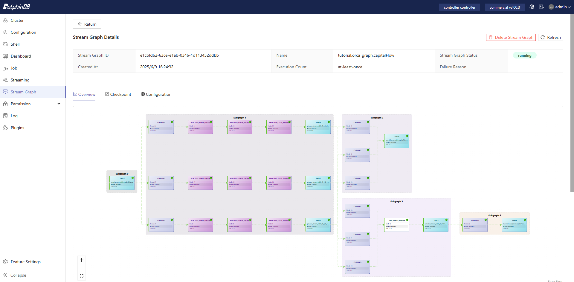
Capital flow computation represents a multi-step cascaded stream processing task. Orca automatically distributes tasks to relatively idle nodes based on the load across the cluster, achieving load balancing. Simultaneously, cluster mode provides high-availability functionality for stream computing tasks, meeting production requirements.
3.4 Data Replay
useOrcaStreamTable("tutorial.orca_table.tradeOriginal", def (table) {
    submitJob("replay", "replay", def (table) {
        ds = replayDS(<select * from loadTable("dfs://trade", `trade) where TradeDate=2024.10.09>, datecolumn=`TradeDate)
        replay(inputTables=ds, outputTables=table, dateColumn=`TradeTime, timeColumn=`TradeTime, replayRate=1, absoluteRate=false, preciseRate=true)
    }, table)
})- Within Orca clusters, stream tables are persisted on data nodes. The system
provides the
useOrcaStreamTablefunction for convenient remote invocation of stream tables on data nodes from compute nodes, including replay operations. When utilizinguseOrcaStreamTable, users need not determine the specific node location of stream tables in advance. - In this example, a background replay task is submitted through
submitJobon the data node containing the tradeOriginal table. The replay task injects data stored in DFS tables into the stream table to simulate real-time market data ingestion.
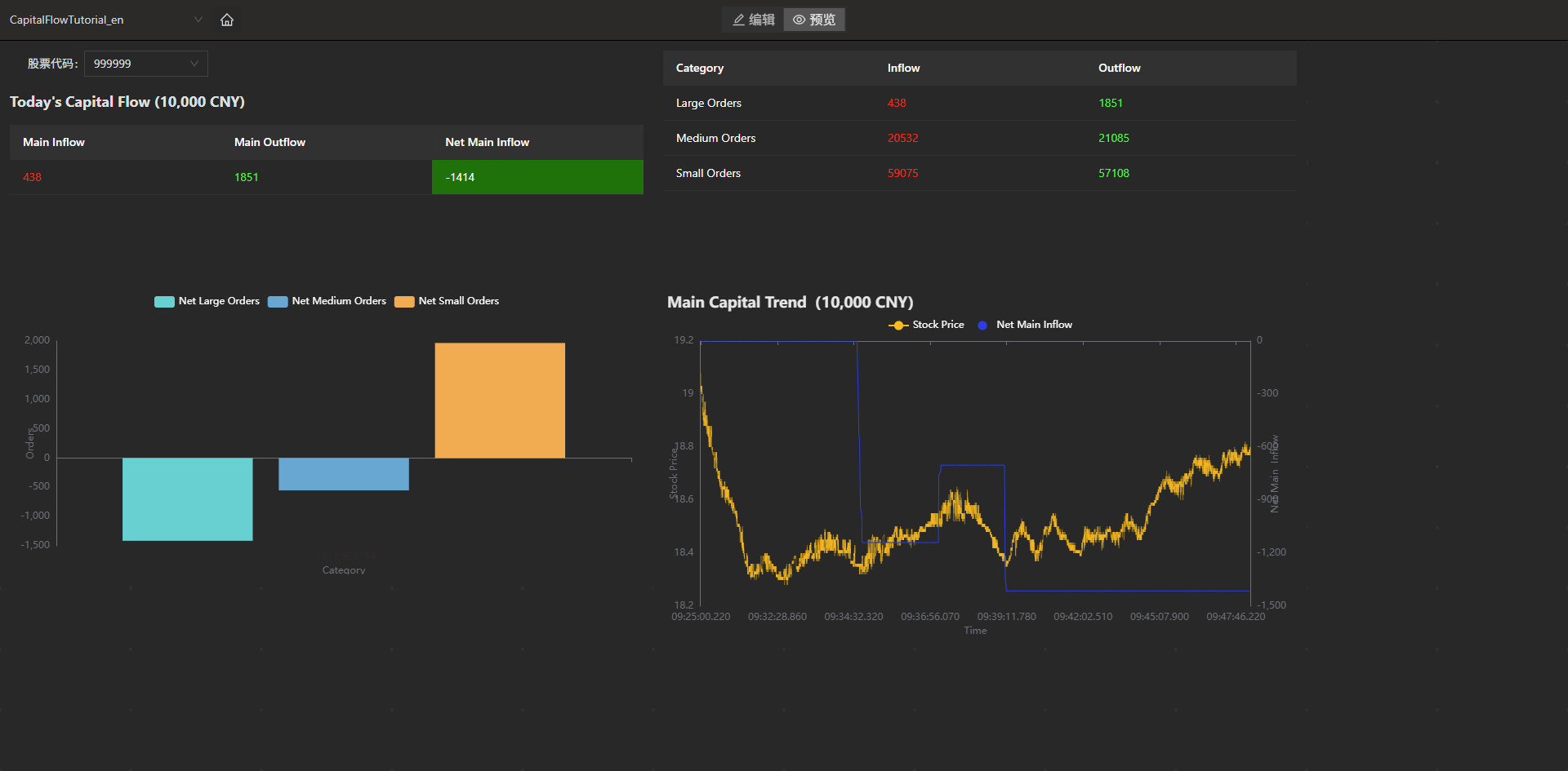
3.5 Dashboard Visualization
For output results, beyond SQL statement querying or API subscriptions, DolphinDB provides a more intuitive presentation solution—Dashboard. Following stream computing job submission, Dashboard updates charts in real-time.
The data panel configuration based on capital flow data computed in this document produces the following effect. The corresponding JSON configuration file is provided in the appendix.
3.6 Advantages of the DStream API
Reviewing this chapter in its entirety, users with experience in DolphinDB's traditional Stream API can clearly observe the usability improvements delivered by DStream API. DStream API, through its method chaining programming style, simplifies stream computing framework construction processes, enabling users to focus on business logic implementation. Primary optimizations include:
Enhanced development efficiency
- Complete data transformation logic including engine cascading through method chaining, aligning with conventional cognitive patterns.
- Automatic inference of result fields and field types from various transformations, eliminating manual specification and reducing verbose table creation statements in script development.
- Rapid parallel computing definition through
DStream::syncandDStream::parallelizemethods, eliminating manual job partitioning and consumption thread specification. - Highly abstracted interfaces eliminate user concern for underlying mechanisms such as shared session management and consumption thread allocation.
Improved operational efficiency
- Catalog enables systematic management of data and jobs across different users, projects, and asset types
- Stream graph for complete stream computing job description enhances job management convenience. During maintenance phases, stream computing job boundaries are clearly defined. Additionally, stream graph release enables rapid resource cleanup for associated stream computing engines and stream tables.
- Enhanced job management visualization through web interfaces providing comprehensive stream computing job (stream graph) management capabilities. Complex interdependencies among engines, stream data tables, subscriptions, and parallelism automatically generate DAG visualizations for web presentation following script submission
Beyond development and operational efficiency improvements, Orca implements further enhancements in automatic scheduling and computing high availability compared to previous versions.
4. Performance Testing
This chapter evaluates response latency for individual records by replaying tick-by-tick data from 100 securities at original speed on 2024.10.09, comparing the performance characteristics of DStream API and traditional Stream API implementations.
4.1 Performance Results
Statistics were collected on single response computation time, defined as the duration from the 1st reactive state engine receiving input to the 3rd reactive state engine producing output, during which 12 indicators across both buy and sell directions are computed. The average response time across all daily output records constitutes the performance evaluation results.
| Implementation Method | Single Response Computation Time (ms) |
|---|---|
| Orca DStream API | 0.238 ms |
| Traditional Stream API | 0.247 ms |
DStream API maintains essentially equivalent computational performance to traditional Stream API while providing highly abstracted and concise programming interfaces, sustaining sub-millisecond processing performance primarily attributed to DolphinDB's stream computing engine and incremental operators.
4.2 Test Environment Configuration
DolphinDB server installation configured in cluster mode. Hardware and software environments for this evaluation are specified below:
Hardware Environment
| Component | Specification |
|---|---|
| Kernel | 3.10.0-1160.88.1.el7.x86_64 |
| CPU | Intel(R) Xeon(R) Gold 5220R CPU @ 2.20GHz |
| Memory | 16 × 32GB RDIMM, 3200 MT/s (Total: 512GB) |
Software Environment
| Component | Version and Configuration |
|---|---|
| Operating System | CentOS Linux 7 (Core) |
| DolphinDB | Server Version: 3.00.3 2025.05.15 LINUX x86_64 |
| License Limit: 16 cores, 512GB memory | |
| Max memory available per test node: 232GB (configured) |
5. Conclusion
This tutorial presented the capabilities of the Orca DStream API through two progressively complex examples, demonstrating its power and practicality in stream processing:
- Conciseness: Developers can focus on business logic without the need to manually create stream tables or cascade engines.
- High-level abstraction: System implementation details are abstracted through the declarative interfaces.
The declarative stream processing interface provided by Orca delivers robust support for DolphinDB applications in enterprise-grade real-time computing environments. In subsequent releases, Orca will continue expanding DStream API operator functionality, enhancing expressive capabilities to assist users in addressing complex real-time computing scenarios.
Appendix
- Sample data: trade.csv
- Database and table creation with sample data import script: CreateDB&LoadText.dos
- Quick start: 5-minute active trading volume ratio script: QuickStart.dos
- Application case: Real-time daily cumulative order-by-order capital flow script: CapitalFlow.dos
- Dashboard configuration: dashboard.CapitalFlowTutorial.json