Empyrical Module for Risk and Performance Metrics
The Empyrical library is an open-source Python library developed by Quantopian, specifically designed for calculating commonly used financial risk and performance attribution metrics. It includes a variety of tools for strategy backtesting analysis and can be used to compute metrics such as annualized return, maximum drawdown, alpha, beta, Calmar ratio, Omega ratio, and Sharpe ratio. To facilitate the calculation of these metrics in DolphinDB, we have implemented the metric functions from the Empyrical library using DolphinDB scripts and encapsulated them in the DolphinDB Empyrical module.
1. Naming and Parameter Conventions
All function names in the Empyrical module follow the convention of using the
specific function's purpose as its name, such as simpleReturns,
cumReturns, cumMaxDrawdown,
calmarRatio, sharpeRatio,
rollSharpeRatio, alpha, etc.
All fields involved in this tutorial are as follows:
| Parameter / Field | Description |
|---|---|
| prices | Closing prices |
| returns | Daily simple (non-cumulative) returns |
| factorReturns | Benchmark returns / factor returns for comparison |
| factorLoadings | Factor loadings |
Note:
- In the
perfAttribfunction, factorReturns refers to the factor returns of different factors and is input as a multi-column table. - The returns parameter also accepts a benchmark return vector as the input.
- Since the
betafunction conflicts with a built-in function in DolphinDB, the corresponding function in Empyrical is namedcovarBeta(as Empyrical calculates beta using covariance / variance, whereas DolphinDB’sbetarefers to the least squares estimate of Y regressed on X). - In DolphinDB, the
maxDrawdownfunction calculates the maximum difference from a peak. In the Empyrical library, the function is defined as the cumulative maximum relative drawdown. Due to the naming conflict, the function that calculates maximum drawdown in Empyrical is namedcumMaxDrawdown. - The function
valueAtRiskhas the same meaning in both DolphinDB and Empyrical. In the Empyrical library, we use the historical simulation method to compute Value at Risk. Due to the naming conflict, the corresponding function in Empyrical is namedhisValueAtRisk.
2. Usage Examples
This chapter introduces the usage of Empyrical module, including environment setup, data preparation and function calls.
2.1 Environment Setup
Place the attached Empyrical.dos file in the [home]/modules
directory. The [home] directory is set by the system configuration
parameter home, which can be viewed using the
getHomeDir() function.
For details on module usage, see Tutorial > Modules.
2.2 Direct Function Call
Call the sharpeRatio function on a vector:
use Empyrical
ret = 0.072 0.0697 0.08 0.74 1.49 0.9 0.26 0.9 0.35 0.63
x = sharpeRatio(ret);
2.3 Grouped Calculation in SQL Statements
To perform grouped calculations, we can call the function in the SQL statement.
For example, the table t contains data for 2 stocks:
close = 7.2 6.97 7.08 6.74 6.49 5.9 6.26 5.9 5.35 5.63 3.81 3.935 4.04 3.74 3.7 3.33 3.64 3.31 2.69 2.72
date = (2023.03.02 + 0..4 join 7..11).take(20)
symbol = take(`F,10) join take(`GPRO,10)
t = table(symbol, date, close)
Calculate the return for each stock:
update t set ret = simpleReturns(close) context by symbol2.4 Functions With Multiple Returns
Functions such as alphaBeta return multiple columns of results.
For example:
use Empyrical

ret = 0.072 0.0697 0.08 0.74 1.49 0.9 0.26 0.9 0.35 0.63
factorret = 0.702 0.97 0.708 1.74 0.49 0.09 1.26 0.59 1.35 0.063
alpha, beta = alphaBeta(ret, factorret);
Use in a SQL statement:
use Empyrical

ret = 0.072 0.0697 0.08 0.74 1.49 0.9 0.26 0.9 0.35 0.63 0.702 0.97 0.708 1.74 0.49 0.09 1.26 0.59 1.35 0.063
factorret = 0.702 0.97 0.708 1.74 0.49 0.09 1.26 0.59 1.35 0.063 0.072 0.0697 0.08 0.74 1.49 0.9 0.26 0.9 0.35 0.63
symbol = take(`F,10) join take(`GPRO,10)
date = (2022.03.02 + 0..4 join 7..11).take(20)
t = table(symbol as sym, date as dt, ret, factorret)
select sym,alphaBeta(ret, factorret) as `alpha`beta from t context by sym

/*
sym  alpha                beta
---- -------------------- ------------------
F    2.936093190579921E62 -0.276883617899559
F    2.936093190579921E62 -0.276883617899559
...
*/
3. Function Performance Evaluation
This section uses the rollSharpeRatio function as an example to
conduct a performance comparison of direct function call, and also provides the
performance comparison of all functions in grouped use in SQL statements using real
daily stock return data.
3.1 Direct Function Call
use Empyrical

ret= 0.072 0.0697 0.08 0.74 1.49 0.9 0.26 0.9 0.35 0.63
ret = take(ret, 10000000)
timer x = rollSharpeRatio(ret, windows =10)
Applying the rollSharpeRatio function from the Empyrical module
directly on a vector of length 10,000,000 took 300.135 ms.
The corresponding Python code is as follows:
import numpy as np
import empyrical as em
import time
ret = np.array([0.072, 0.0697, 0.08, 0.74, 1.49, 0.9, 0.26, 0.9, 0.35, 0.63])
ret = np.tile(ret,10000000)
start_time = time.time()
x = em.roll_sharpe_ratio(ret, 10)
print("--- %s seconds ---" % (time.time() - start_time))
The roll_sharpe_ratio function from the Python Empyrical library
took 25,965.46 ms, which is 86 times longer than the
rollSharpeRatio function in the DolphinDB Empyrical
module.
3.2 Grouped Calculation in SQL Statements
The performance test data consists of daily return data for all stocks in market
from January 3, 2019, to July 1, 2022, along with simulated factor data and
portfolio weights (for testing computeExposure and
perfAttrib functions), totaling 3,452,106 records. Sample
data from the test files are provided in the appendix. After extraction, place
them under the [home] directory.
The computation logic involves grouping by stock code to calculate each metric. To evaluate the function performance, both the DolphinDB and Python test codes are executed in single-threaded mode.
The test result is as shown in the table:
| No. | Function | DolphinDB Time | Python Time | Python/DolphinDB |
|---|---|---|---|---|
| 1 | simpleReturns | 190.7 ms | 5,871.1ms | 30.78 |
| 2 | aggregateReturns | 238.5 ms | 11,167.8 ms | 46.83 |
| 3 | annualReturns | 66.8 ms | 889.1ms | 13.30 |
| 4 | cumReturns | 84.7 ms | 2,758.7ms | 32.56 |
| 5 | cumReturnsFinal | 82.4 ms | 835.4ms | 10.13 |
| 6 | alpha | 131.2 ms | 6,910.7 ms | 52.67 |
| 7 | rollAlpha | 548.1 ms | 5,143.4 ms | 9.38 |
| 8 | covarBeta | 84.3ms | 5,422.9 ms | 64.32 |
| 9 | rollCovarBeta | 195.9 ms | 4,306.8 ms | 21.98 |
| 10 | alphaBeta | 112.5 ms | 6,929.8 ms | 61.59 |
| 11 | rollAlphaBeta | 547.7 ms | 8,676.7 ms | 15.84 |
| 12 | upAlphaBeta | 156.1 ms | 5,653.1 ms | 36.21 |
| 13 | downAlphaBeta | 148.6 ms | 5,722.9 ms | 38.52 |
| 14 | betaFragilityHeuristic | 262.7 ms | 12,906.5 ms | 49.14 |
| 15 | annualVolatility | 64.5 ms | 776.5 ms | 12.03 |
| 16 | rollAnnualVolatility | 136.9 ms | 2,869.9 ms | 20.96 |
| 17 | downsideRisk | 137.3 ms | 679.0 ms | 4.94 |
| 18 | hisValueAtRisk | 152.9 ms | 710.3 ms | 4.64 |
| 19 | conditionalValueAtRisk | 155.8 ms | 306.2 ms | 1.97 |
| 20 | gpdRiskEstimates | 7.3s | 26.4s | 3.61 |
| 21 | tailRatio | 235.4 ms | 1,224.2 ms | 5.20 |
| 22 | capture | 103.7 ms | 2,343.0 ms | 22.59 |
| 23 | upCapture | 165.7 ms | 4,284.7 ms | 25.69 |
| 24 | downCapture | 165.6 ms | 4,254.3 ms | 25.85 |
| 25 | upDownCapture | 232.8 ms | 7,380.0 ms | 31.70 |
| 26 | rollUpCapture | 30.1 s | 2,204.8 s | 73.33 |
| 27 | rollDownCapture | 30.4 s | 2,195.3 s | 72.32 |
| 28 | rollUpDownCapture | 53.7 s | 4,146.4 s | 77.20 |
| 29 | omegaRatio | 111.6 ms | 3,946.0 ms | 35.37 |
| 30 | cumMaxDrawdown | 99.4 ms | 500.3ms | 5.03 |
| 31 | rollCumMaxDrawdown | 1.4s | 3.1s | 2.11 |
| 32 | calmarRatio | 118.3 ms | 1,338.4 ms | 11.32 |
| 33 | sharpeRatio | 100.6 ms | 974.7 ms | 9.68 |
| 34 | rollSharpeRatio | 160.7 ms | 3,277.3 ms | 20.39 |
| 35 | excessSharpe | 103.6 ms | 2,828.9 ms | 27.31 |
| 36 | sortinoRatio | 180.5 ms | 988.8 ms | 5.47 |
| 37 | rollSortinoRatio | 287.0 ms | 3,160.3 ms | 11.01 |
| 38 | stabilityOfTimeseries | 365.5 ms | 1,707.9 ms | 4.67 |
| 39 | computeExposure | 183.6 ms | 256.5 ms | 1.39 |
| 40 | perfAttrib | 251.9 ms | 3,484.8 ms | 13.83 |
The test results show that the function performance of the DolphinDB Empyrical module surpasses that of the Python Empyrical library in most cases, with the maximum performance gap reaching 70 times, and an average gap of around 9 times.
Python pandas test code:
grouped = returns.groupby('SecurityID')
cum_returns = grouped['ret'].apply(lambda x: em.cum_returns(x))
DolphinDB test code:
cumReturns =
    select SecurityID, DateTime, cumReturns(ret) as cumReturns
    from returns
    context by SecurityID
4. Consistency Verification
Based on the test data and code used in the performance comparison for grouped calculation, we also verify whether the calculation results of functions in the DolphinDB Empyrical module are consistent with those in the Python Empyrical library.
4.1 Handling of Null Values
If the input vector in Python Empyrical contains null values, the nulls are passed into the function and included in the calculation. The Empyrical module adopts the same strategy. The results produced by DolphinDB Empyrical are closely aligned with those of the Python Empyrical library, with only minor differences due to floating-point precision.
Note: While DolphinDB retains null values at the first (k–1) positions for strict window alignment, the Python Empyrical library skips initial nan values and begins computation as soon as a valid window is available.
DolphinDB Example
ret = NULL NULL 0.08 0.74 1.49 0.9 0.26 0.9 0.35 0.63 0.702 0.97 0.708 1.74
0.49 0.09 1.26 0.59 1.35 0.063
rollAnnualVolatility(ret, windows =10)

/*
[,,,,,,,,,7.107626186006128,6.650903096572676,6.445987651244765,5.4412961691126505,
7.3080574710383885,6.603612950499143,7.349681897878303,7.448075187590415,
7.475411961892134,7.649430305584855,8.584637604465316]
*/
Python Example
ret = np.array([np.nan, np.nan, 0.08, 0.74, 1.49, 0.9, 0.26,
0.9, 0.35, 0.63, 0.702, 0.97, 0.708, 1.74, 0.49, 0.09, 1.26, 0.59, 1.35, 0.063])
print(em.roll_annual_volatility(ret,10))

/*
[7.10762619 6.6509031  6.44598765 5.44129617 7.30805747 6.60361295
 7.3496819  7.44807519 7.47541196 7.64943031 8.5846376 ]
 */
4.2 Optimized Output Format
The following functions generate different results from Python:
alphaBeta, upAlphaBeta,
downAlphaBeta, gpdRiskEstimates.
In Python Empyrical, the results of alphaBeta,
upAlphaBeta, and downAlphaBeta combine
alpha and beta into a two-dimensional array, requiring further post-processing.
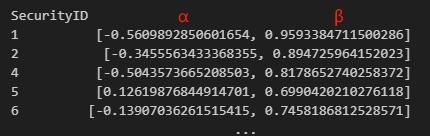
In DolphinDB, alpha and beta can be directly separated into two columns using SQL query statements.
select SecurityID, alphaBeta(ret, factorRet) as `alpha`beta
from return1
group by SecurityID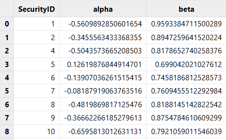
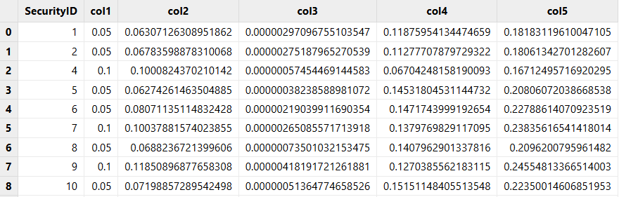
While for the function gpdRiskEstimates, all the estimates are
output in one column in Python:
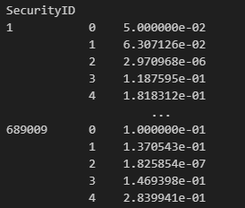
In DolphinDB, the estimates are displayed in separate columns:
5. Real-Time Stream Processing
Most functions in the Empyrical module can be used in the reactive state engine as metrics for real-time incremental calculation. For example:
// clean environment
def cleanEnvironment(){
    try{ unsubscribeTable(tableName="inputTable",actionName="calculateEmpyrical") }
    catch(ex){ print(ex) }
    try{ dropStreamEngine("EmpyricalReactiveSateEngine") } catch(ex){ print(ex) }
    try{ dropStreamTable(`inputTable) } catch(ex){ print(ex) }
    try{ dropStreamTable(`outputTable) } catch(ex){ print(ex) }
    undef all
}
cleanEnvironment()
go

// load module
use Empyrical

// load data
schema = table(`DateTime`SecurityID`ret`factor2`factor1`factor3`position as name,
`DATE`SYMBOL`DOUBLE`DOUBLE`DOUBLE`DOUBLE`DOUBLE as type)
data=loadText(<YOUR_DIR>+"factors_data.csv" ,schema=schema)
// define stream table
share streamTable(1:0, `DateTime`SecurityID`ret`factor2`factor1`factor3`position,
`DATE`SYMBOL`DOUBLE`DOUBLE`DOUBLE`DOUBLE`DOUBLE) as inputTable
share streamTable(1:0,`SecurityID`DateTime`sortinoRatio`annualVolatility`sharpeRatio,
`SYMBOL`DATE`DOUBLE`DOUBLE`DOUBLE) as outputTable

// register stream computing engine
reactiveStateMetrics=<[
    DateTime,
    Empyrical::rollAnnualVolatility(ret) as `sortinoRatio,
    Empyrical::rollSharpeRatio(ret) as `annualVolatility,
    Empyrical::rollSortinoRatio(ret) as `sharpeRatio
]>
createReactiveStateEngine(name="EmpyricalReactiveSateEngine",
metrics=reactiveStateMetrics, dummyTable=inputTable, outputTable=outputTable,
keyColumn=`SecurityID, keepOrder=true)
subscribeTable(tableName="inputTable", actionName="calculateEmpyrical",
offset=-1, handler=getStreamEngine("EmpyricalReactiveSateEngine"),
msgAsTable=true, reconnect=true)
// replay data
submitJob("replay","replay",replay{data,inputTable,`tradedate,`tradedate,1000,true})
6. Empyrical Function Reference
6.1 Returns
| Function | Syntax | Description |
|---|---|---|
| simpleReturns | simpleReturns(prices) | Simple returns |
| aggregateReturns | aggregateReturns(returns,date, convertTo='yearly') | Aggregate returns by week, month, or year |
| annualReturns | annualReturn(returns, period="daily", annualization=NULL) | Compound annual growth rate (CAGR) |
| cumReturns | cumReturns(returns, startingValue=0) | Cumulative simple returns |
| cumReturnsFinal | cumReturnsFinal(returns, startingValue=0) | Total simple returns |
6.2 Alpha & Beta
| Function | Syntax | Description |
|---|---|---|
| alpha | alpha(returns, factorReturns, riskFree=0.0, period="daily", annualization=NULL, beta=NULL) | Annualized alpha |
| rollAlpha | rollAlpha(returns, factorReturns, riskFree=0.0, period="daily", annualization=NULL, windows = 10) | Rolling window alpha |
| covarBeta | covarBeta(returns, factorReturns, riskFree=0.0) | Beta value |
| rollCovarBeta | rollCovarBeta(returns, factorReturns, riskFree=0.0, windows = 10) | Rolling window beta |
| alphaBeta | alphaBeta(returns, factorReturns, riskFree=0.0, period="daily", annualization=NULL) | Annualized alpha and beta |
| rollAlphaBeta | rollAlphaBeta(returns, factorReturns, riskFree=0.0, period="daily", annualization=NULL, windows=10) | Rolling window alpha and beta |
| upAlphaBeta | upAlphaBeta(returns, factorReturns, riskFree=0.0, period="daily", annualization=NULL) | Alpha and beta during periods of positive benchmark returns |
| downAlphaBeta | downAlphaBeta(returns, factorReturns, riskFree=0.0, period="daily", annualization=NULL) | Alpha and beta during periods of negative benchmark returns |
| betaFragilityHeuristic | betaFragilityHeuristic(returns, factorReturns) | Estimate fragility when beta declines |
6.3 Risk Management
| Function | Syntax | Description |
|---|---|---|
| annualVolatility | annualVolatility(returns, period="daily", annualization=NULL, alpha=2.0) | Annualized volatility |
| rollAnnualVolatility | rollAnnualVolatility(returns, period="daily", annualization=NULL, windows=10, alpha=2.0) | Rolling window annualized volatility |
| downsideRisk | downsideRisk(returns, requiredReturn=0.0, period="daily", annualization=NULL) | Downside deviation below a threshold |
| hisValueAtRisk | valueAtRisk(returns, cutoff=0.05) | Value at risk (VaR) |
| conditionalValueAtRisk | conditionalValueAtRisk(returns, cutoff=0.05) | Conditional value at risk (CVaR) |
| gpdRiskEstimates | gpdRiskEstimates(returns, varP=0.01) | Estimate VaR and ES using generalized pareto distribution (GPD) |
| tailRatio | tailRatio(returns) | Ratio between the right tail (95%) and the left tail (5%) |
6.4 Capture Ratio
| Function | Syntax | Description |
|---|---|---|
| capture | capture(returns, factorReturns, period="daily", annualization=NULL) | Capture ratio |
| upCapture | upCapture(returns, factorReturns, period="daily", annualization=NULL) | Up capture ratio during periods of positive benchmark returns |
| downCapture | downCapture(returns, factorReturns, period="daily", annualization=NULL) | Up capture ratio during periods of negative benchmark returns |
| upDownCapture | upDownCapture(returns, factorReturns, period="daily", annualization=NULL) | Ratio of up capture to down capture |
| rollUpCapture | rollUpCapture(returns, factorReturns, windows=10, period="daily", annualization=NULL) | Rolling up capture ratio |
| rollDownCapture | rollDownCapture(returns, factorReturns, windows=10, period="daily", annualization=NULL) | Rolling down capture ratio |
| rollUpDownCapture | rollUpDownCapture(returns, factorReturns, windows=10, period="daily", annualization=NULL) | Ratio of rolling up capture to rolling down capture |
6.5 Risk-Adjusted Returns
| Function | Syntax | Description |
|---|---|---|
| omegaRatio | omegaRatio(returns, period="daily", riskFree=0.0, requiredReturn=0.0, annualization=NULL) | Omega ratio |
| cumMaxDrawdown | maxdrawdown(returns) | Maximum drawdown |
| rollCumMaxDrawdown | rollCumMaxDrawdown(returns, windows = 10) | Rolling window maximum drawdown |
| calmarRatio | calmarRatio(returns, period="daily", annualization=NULL) | Calmar ratio of the strategy, i.e., drawdown ratio |
| sharpeRatio | sharpeRatio(returns, riskFree=0.0, period="daily", annualization=NULL) | Sharpe ratio |
| rollSharpeRatio | rollSharpeRatio(returns, riskFree=0.0, period="daily", annualization=NULL, windows=10) | Rolling Sharpe ratio |
| excessSharpe | excessSharpe(returns, factorReturns) | Excess Sharpe ratio |
| sortinoRatio | sortinoRatio(returns, requiredReturn=0.0, period="daily", annualization=NULL) | Sortino ratio |
| rollSortinoRatio | rollSortinoRatio(returns, requiredReturn=0.0, period="daily", annualization=NULL, windows=10) | Rolling Sortino ratio |
6.6 Return Stability and Performance Attribution
| Function | Syntax | Description |
|---|---|---|
| stabilityOfTimeseries | stabilityOfTimeseries(returns) | R² of the linear fit to cumulative log returns |
| computeExposure | computeExposures( factorLoadings, factorColumns=`factor1`factor2`factor3, positionName=`position`position`position, dtName=`DateTime) | Daily risk factor exposures |
| perfAttrib | perfAttrib(returns, factorReturns, factorLoadings, factorColumns=`factor1`factor2`factor3, positionName=`position`position`position, dtName=`DateTime) | Performance attribution (attributing investment returns to a set of risk factors) |