Data Partitioning

Range partitioning is suitable for storing time series data, or continuous numerical data. Partitions of the RANGE type are defined by ranges where the boundaries are two consecutive elements from the partition scheme vector. The starting value is inclusive, while the ending value is exclusive.

For example, to create a database db with 2 partitions: [0,5) and [5,10), specify partitionScheme = 0 5 10. Then, create a partitioned table with the partitioning column ID in db.

n=1000000
ID=rand(10, n)
x=rand(1.0, n)
t=table(ID, x)
db=database("dfs://rangedb", RANGE,  0 5 10)

pt = db.createPartitionedTable(t, `pt, `ID)
pt.append!(t)

pt=loadTable(db,`pt)
select count(x) from pt;

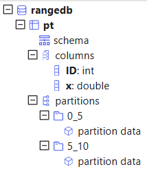
Once data is appended to pt, the system will organize it based on the ID values: records with ID values ranging from 0 to 4 will be stored in partition 0_5 and 5 to 9 in 5_10.

Note: The partition scheme of a range-partitioned database can be appended after it is created. See function addRangePartitions for details.

Hash partitioning creates a specified number of partitions using a hash function on the partitioning column. This method helps balance data distribution, reducing the risk of overloaded partitions. However, it may still result in uneven partition sizes if the partitioning column values are skewed. For efficient retrieval of data within a range, range or value partitions are preferable to hash partitions.

For example, to create a database db with 2 partitions based on an INT column, specify partitionScheme = [INT, 2]. Then, create a partitioned table with the partitioning column ID in db.

n=1000000
ID=rand(10, n)
x=rand(1.0, n)
t=table(ID, x)
db=database("dfs://hashdb", HASH,  [INT, 2])

pt = db.createPartitionedTable(t, `pt, `ID)
pt.append!(t)

pt=loadTable(db,`pt)
select count(x) from pt;

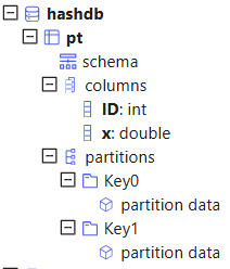
Once data is appended to pt, the system will organize it based on hash values. Records sharing the same hash value are grouped into the same partition (e.g., Key0, Key1).

Value partitioning creates partitions based on specific values in the partitioning column, typically applied to date and time columns (see section Partitions on Temporal Values).

For example, to create a database db with 204 monthly partitions from January 2000 to December 2016, specify partitionScheme as a vector, 2000.01M..2016.12M, with each element corresponding to a partition. Then, create a partitioned table with the partitioning column month in db.

n=1000000
month=take(2000.01M..2016.12M, n)
x=rand(1.0, n)
t=table(month, x)

db=database("dfs://valuedb", VALUE, 2000.01M..2016.12M)

pt = db.createPartitionedTable(t, `pt, `month)
pt.append!(t)

pt=loadTable(db,`pt)
select count(x) from pt;

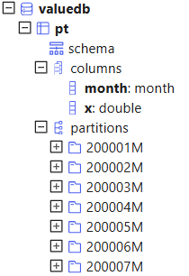
Once data is appended to pt, the system will organize it based on month. For example, data in 2000.01 will be stored in 200001M.

Note: The partition scheme of a value-partitioned database can be appended after it is created. See function addValuePartitions and configuration parameter newValuePartitionPolicy for details.

List partitioning partitions data based on specified sets of enum values. It's particularly useful when you need to include multiple partitioning column values into a single partition.

Note: The difference between the list type and value type is that all the elements in a value partition scheme are scalars, whereas each element in a list partition scheme may be a vector.

For example, to create a database db with 2 partitions based on symbol, specify partitionScheme as a vector, [`IBM`ORCL`MSFT, `GOOG`FB], with each element grouped into a partition. Then, create a partitioned table with the partitioning column “ticker” in db.

n=1000000
symbol = rand(`MSFT`GOOG`FB`ORCL`IBM,n)
x=rand(1.0, n)
t=table(symbol, x)

db=database("dfs://listdb", LIST, [`IBM`ORCL`MSFT, `GOOG`FB])
pt = db.createPartitionedTable(t, `pt, `symbol)
pt.append!(t)

pt=loadTable(db,`pt)
select count(x) from pt;

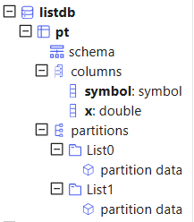
Once data is appended to pt, the system will automatically organize it based on symbol: records with symbol=`IBM`ORCL`MSFT are stored in List0 and symbol=`GOOG`FB in List1.

Composite partitioning allows for flexible, multi-dimensional data organization.

For example, to create a database db based on 2-dimension partitioning, specify partitionScheme as a vector, [dbDate, dbID], with each element corresponding to a database handle. dbDate is value-partitioned and dbID is range-partitioned. Then, create a partitioned table with partitioning columns “date” and “ID“ in db.

n=1000000
ID=rand(100, n)
dates=2017.08.07..2017.08.11
date=rand(dates, n)
x=rand(10.0, n)
t=table(ID, date, x)

dbDate = database(, VALUE, 2017.08.07..2017.08.11)
dbID=database(, RANGE, 0 50 100)
db = database("dfs://compoDB", COMPO, [dbDate, dbID])

pt = db.createPartitionedTable(t, `pt, `date`ID)
pt.append!(t)

pt=loadTable(db,`pt)
select count(x) from pt;

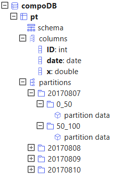
Once data is appended to pt, the system will organize it along both dimensions: VALUE+RANGE. The value domain has 5 partitions. Click on a date partition, we can see the range domain has 2 partitions:

Note: If one of the partitioning columns is of value domain, it can be appended with new values after it is created. See function addValuePartitions and configuration parameter newValuePartitionPolicy for details.

DolphinDB provides a custom solution for data partitioning based on user-defined rules to flexibly accommodate diverse partitioning requirements. For example:

• Applying prefix functions to futures and options contract data from exchanges;
• Partitioning based on IoT metric IDs;
• Extracting date and time information from encoded data.

The parameter partitionColumns of createPartitionedTable function and create statement supports specifying a user-defined function to a column and using the transformed result as a partitioning column.

For instance, for data with a column in the format id_date_id (e.g., ax1ve_20240101_e37f6), users can partition by date using a user-defined function:

// Define a function to extract the date information
def myPartitionFunc(str,a,b) {
    return temporalParse(substr(str, a, b),"yyyyMMdd")
}

// Create a database
data = ["ax1ve_20240101_e37f6", "91f86_20240103_b781d", "475b4_20240101_6d9b2", "239xj_20240102_x983n","2940x_20240102_d9237"]
tb = table(data as id_date, 1..5 as value, `a`b`c`d`e as sym)
db = database("dfs://testdb", VALUE, 2024.02.01..2024.02.02)

// Use myPartitionFunc to process the data column
pt = db.createPartitionedTable(table=tb, tableName=`pt, 
    partitionColumns=["myPartitionFunc(id_date, 6, 8)"])
pt.append!(tb)

select * from pt

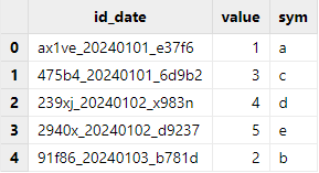
Records queried by the select statement are read and returned by partition. The query result shows that table pt is partitioned by the date information extracted from the id_date column.

When implementing partitions in a database, the choice of partitioning column(s) is a crucial decision made during table creation. This choice significantly affects subsequent data operations, especially queries involving or related to the partitioning columns.

Supported Data Types

In DolphinDB, the data types that can be used for partitioning columns include integers (CHAR, SHORT, INT), temporal (DATE, MONTH, TIME, SECOND, MINUTE, DATETIME, DATEHOUR), STRING and SYMBOL. The HASH domain also supports LONG, UUID, IPADDR and INT128 types. Although a partitioning column can be of STRING type, for optimal performance, we recommend converting a STRING type column into SYMBOL type to be used as a partitioning column.

FLOAT and DOUBLE types cannot be used as a partitioning column.

db=database("dfs://rangedb1", RANGE,  0.0 5.0 10.0);
// report an error
The data type DOUBLE can't be used for a partition column.

Select Columns Frequently Used

Select partitioning columns that align with frequent database updates in your business context. For example, many tasks on financial databases involve stock symbols and dates. Therefore stock symbols and dates are natural candidates as partitioning columns.

Note: DolphinDB doesn't allow multiple threads or processes to write to the same partition simultaneously when updating the database. Considering we may need to update data of a date or of a stock, if we use other partitioning columns such as trading hour, multiple writers may write to the same partition simultaneously and cause problems.

Additionally, a partitioning column is equivalent to a physical index on a table. If a query uses a partitioning column in where conditions, the system can quickly load the target data instead of scanning the entire table. Therefore, partitioning columns should be the columns that are frequently used in where conditions for optimal performance.

The columns in a partition are stored as separate files on disk after compression. When a query reads the partition, the system loads the necessary columns into memory after decompression. Too large partitions may slow down the system, as they may cause insufficient memory with multiple threads running in parallel, or they may make the system swap data between disk and memory too frequently. As a rule of thumb, assume the available memory of a data node is S and the number of workers is W, then it is recommended that a partition is less than S/8W in memory after decompression，For example, with available memory of 32GB and 8 workers, a single partition should be smaller than 32GB/8/8=512MB.

The number of subtasks of a query is the same as the number of partitions involved. Therefore if partitions are too large, the system cannot fully take advantage of distributed computing on multiple partitions.

DolphinDB is designed as an OLAP database system. It supports appending data to tables, but does not support deleting or modifying individual rows. To modify certain rows, we need to overwrite entire partitions containing these rows. If the partitions are too large, it would be too slow to modify data. When we copy or move selected data between nodes, entire partitions with the selected data are copied or moved. If the partitions are too large, it would be too slow to copy or move data.

Considering all the factors mentioned above, we recommend the size of a partition does not exceed 1GB before compression. This restriction can be adjusted based on the specific situations. For example, when we work with a table with hundreds of columns and only a small subset of columns are actually used, we can relax the upper limit of the partition size range.

To reduce partitions sizes, we can (1) use composite partitions (COMPO); (2) increase the number of partitions; (3) use value partitions instead of range partitions.

If partition size is too small, a query or computing job may generate a large number of subtasks. This increases the time and resources in communicating between the controller node and data nodes, and between different controller nodes. Too small partitions also result in innefficient reading/writing of small files on disk and therefore. Lastly, the metadata of all partitions are stored in the memory of the controller node. Too many small partitions may make the controller node run out of memory. We recommend that the partition size is larger than 100 MB on average before compression. Based on the above-mentioned analysis, we recommend the size of a partition be between 100MB and 1GB.

The distribution of trading activities of stocks is highly skewed. Some stocks are extremely active but a majority of stocks are much less active. For a composite partition with partitioning columns of trading days and stock tickers, if we use value partitions on both partitioning columns, we will have many extremely small partitions for illiquid stocks. In this case we recommend range partitions on stock tickers where many illiquid stocks can be grouped into one partition, resulting a more evenly partitioned dataset for better performance.

Significant differences among partition sizes may cause load imbalance. Some nodes may have heavy workloads while other nodes idle. If a task is divided into multiple subtasks, it returns the final result only after the last subtask is finished. As each subtask works on a different partition, if data is not distributed evenly among partitions, it may increase the execution time.

A useful tool for partitioning data evenly is function cutPoints(X, N, [freq]), where X is a vector; N means the number of buckets the elements of X will be grouped into; the optional argument freq is a vector of the same length as X indicating the frequency of each element in X. It returns a vector with (N+1) elements such that the elements of X are evenly distributed within each of the N buckets indicated by the vector. It can be used to generate the partition scheme of a range domain in a distributed database.

In the following example, we construct a composite partition on date and symbols for high frequency stock quotes data. We use the data of 2007.08.01 to determine 128 stock symbol ranges with equal number of rows on 2007.08.01, and apply these ranges on the entire dataset.

t = ploadText(WORK_DIR+"/TAQ20070801.csv")
t = select count(*) as ct from t where date=2007.08.01 group by symbol
buckets = cutPoints(t.symbol, 128, t.ct)

dateDomain = database("", VALUE, 2017.07.01..2018.06.30)
symDomain = database("", RANGE, buckets)
stockDB = database("dfs://stockDBTest", COMPO, [dateDomain, symDomain]);

In the following example, we create a distributed database with a value partition on date. The partitioning scheme extends to the year 2030 to accommodate updates in future time periods.

dateDB = database("dfs://testDate", VALUE, 2000.01.01 .. 2030.01.01)

When using a time column as the partitioning column, the data type of the partition scheme does not need to be the same as the data type of a partitioning column. For example, if we use month as the partition scheme in a value partition, the data type of the partitioning column can be month, date, datetime, timestamp, or nanotimestamp.

Note: While DolphinDB supports TIME, SECOND, and DATETIME for partitioning columns, avoid using them for value partitions. These time types create millions of small partitions, making both creation and querying inefficient.

It may be time consuming to join multiple tables in a distributed database, as the partitions that need to be joined with may be located on different nodes and therefore data need to be copied and moved across nodes. DolphinDB ensures that the same partitions of all the tables in the same distributed database are stored at the same node. This makes it highly efficient to join these tables. DolphinDB does not support joining tables from different partitioned databases.

dateDomain = database("", VALUE, 2018.05.01..2018.07.01)
symDomain = database("", RANGE, string('A'..'Z') join `ZZZZZ)
stockDB = database("dfs://stockDB", COMPO, [dateDomain, symDomain])

quoteSchema = table(10:0, `sym`date`time`bid`bidSize`ask`askSize, [SYMBOL,DATE,TIME,DOUBLE,INT,DOUBLE,INT])
stockDB.createPartitionedTable(quoteSchema, "quotes", `date`sym)

tradeSchema = table(10:0, `sym`date`time`price`vol, [SYMBOL,DATE,TIME,DOUBLE,INT])
stockDB.createPartitionedTable(tradeSchema, "trades", `date`sym)

In the examples above, the distributed tables quotes and trades are located in the same distributed database.