AI DataLoader
In conventional quantitative strategy development, factors are typically generated using third-party tools like Python and stored as files. These factors, such as technical indicators, volatility metrics, and market sentiment measurements, serve as essential inputs for deep learning models. However, the rapid expansion of securities trading and the exponential growth of factor data have highlighted significant challenges in traditional file-based storage approaches:
- Factor Data Size: The massive volume of factor data creates substantial bottlenecks in memory bandwidth and storage capacity.
- Integration and Engineering Complexity: Integrating factor data with deep learning models has become increasingly intricate and resource-intensive.
AI DataLoader aims to enhance factor data management efficiency and simplify interactions
with deep learning models. Specifically, the DDBDataLoader class
manages factor data and streamlines integration with deep learning frameworks, creating
a more efficient and cohesive workflow.
1. Framework
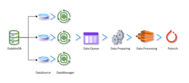
The flow of using DolphinDB with PyTorch involves the following modules:
- Factor data stroage: stores historical factor data in DolphinDB.
- Factor loading: contains the data queue of AI DataLoader
(
DDBDataLoader), which maintains multiple worker threads and message queues internally to enhance concurrent performance. It transforms factor data from DolphinDB into tensors recognizable by deep learning frameworks such as PyTorch, based on a partitioning scheme. Strategy developers can access the required factor data from DolphinDB in real time and push it into deep learning models for training. This real-time capability helps strategy developers obtain the latest data when needed for model training.- First, a
DDBDataLoaderobject is constructed, and queries are divided into several groups based on the data column specified by the groupCol parameter. Within each group query, further subdivision into multiple subqueries is performed according to the data column specified by the repartitionCol parameter. This enhances data flexibility, allowing users to more precisely select the required data to meet deep learning model training needs. - Then the internal threads of the
DDBDataLoaderobject process the partitioned data in background threads by converting and assembling it into the format required for PyTorch training. The processed data is then placed into a prefetch queue. This approach reduces memory consumption on the client side. - The final step involves iteratively retrieving batches of data from the
DDBDataLoaderqueue and returning this data to the client for use in PyTorch training.
- First, a
2. Working Principle
During construction, DDBDataLoader receives a user-provided SQL
query and splits it into multiple subquery groups. DDBDataLoader
uses background threads to fetch data from the server and processes it into batch
data in PyTorch tensors.
DDBDataLoader provides the parameters groupCol and
groupScheme, which are used to split a single SQL query into multiple
query groups. Each group defines a time series, such as the trading data of a single
stock. If not specified, all data is assumed to share a single time series. For
example, a typical case is when the table contains data for all stocks, but during
model training, we only want each stock to use its own historical data for
predicting the future. In this case, we need to set groupCol to the stock
identifier column and groupScheme to all stock identifiers, meaning each
group represents the trading data of one stock. In other words, if the original
query SQL is select * from loadTable(dbName, tableName) and
groupCol is stockID, groupScheme is
["apple", "google", "amazon"], then the original query will be
split into the following three queries:
select * from loadTable(dbName, tableName) where stockID = "apple"
select * from loadTable(dbName, tableName) where stockID = "google"
select * from loadTable(dbName, tableName) where stockID = "amazon"
During model training, each batch of training data will come only from one of the
above groups and will not cross groups. To avoid loading large amounts of data into
memory, DDBDataLoader manages data at the partition level. This
means that for each group, only one partition is loaded into memory at a time.
Typically, a DolphinDB partition is between 100 MB and 1 GB in size, so this design
effectively limits memory usage. On the other hand, this partition-level management
causes the data shuffling implemented by DDBDataLoader to differ
from traditional dataloaders. Specifically, traditional shuffle performs a
completely random shuffle of data, but this introduces a lot of random I/O, reducing
efficiency. DDBDataLoader, however, first randomly selects and
reads a partition, and then performs a shuffle within that partition. This approach
minimizes random I/O as much as possible, improving the efficiency of the overall
training process.
Another set of parameters to explain are repartitionCol and
repartitionScheme. These parameters mainly address the situation where a
single query cannot be directly split into multiple partitions. For example, a
common method of managing factor data in DolphinDB is to use a long table to manage
factor data (see Optimal Storage for Trading Factors Calculated at
Mid to High Frequencies). With this method, before obtaining available
training data, all data needs to be pivoted from long to wide format using
pivot by. However, if the dataset is very large, for example,
several hundred GB or more, the server’s memory may not be sufficient to complete a
pivot by operation on all data. To handle such cases,
DDBDataLoader provides the parameters repartitionCol and
repartitionScheme, which allow further splitting of the entire table into
multiple subtables to be pivoted individually. In other words, if the original query
SQL is select val from loadTable(dbName, tableName) pivot by datetime,
stockID, factorName and repartitionCol
isdate(datetime), repartitionScheme is
["2023.09.05", "2023.09.06", "2023.09.07"], then the above
query would effectively be split into the following subqueries:
select val from loadTable(dbName, tableName) pivot by datetime, stockID, factorName where date(datetime) = 2023.09.05
select val from loadTable(dbName, tableName) pivot by datetime, stockID, factorName where date(datetime) = 2023.09.06
select val from loadTable(dbName, tableName) pivot by datetime, stockID, factorName where date(datetime) = 2023.09.07After setting repartitionCol and repartitionScheme, the pivot
by query result is further repartitioned so that each partition does
not occupy too much memory space.
Within DDBDataLoader, each DataSource functions as metadata for a
partition. A DataSource retrieves data from the DolphinDB server through a session
and places the data into a preloaded queue. DataManager processes the data by
applying specified sliding window size and step, and transforms it into PyTorch
Tensor format.
DDBDataLoader maintains a DataManager pool, with the pool size
controlled by the groupPoolSize parameter. Data is extracted from managers by
background workers, transformed into appropriate training format, and enqueued for
training. DDBDataLoader retrieves processed data from the queue and
delivers them to the client for neural network training. This mechanism ensures that
only one or a few partitions a are read simultaneously, thus reducing memory
consumption.
3. DDBDataLoader
3.1 Installation
Starting from version 1.30.22.2, DolphinDB Python API provides the deep learning
utility class DDBDataLoader , which offers an easy-to-use
interface for batch splitting and reshuffling of datasets corresponding to
DolphinDB SQL, directly integrating data from DolphinDB into PyTorch.
pip install dolphindb-toolsExpected output:

3.2 DolphinDB and Tensor Data Type Mapping
|
DolphinDB Type |
Tensor Type |
|---|---|
| BOOL [null not included] | torch.bool |
| CHAR [null not included] | torch.int8 |
| SHORT [null not included] | torch.int16 |
| INT [null not included] | torch.int32 |
| LONG [null not included] | torch.int64 |
| FLOAT | torch.float32 |
| DOUBLE | torch.float64 |
| CHAR/SHORT/INT/LONG [null included] | torch.float64 |
Note:
- If the result table from the SQL query contains unsupported types, even if the column names are specified in targetCol (which indicates the column names corresponding to y during iteration), those data columns will not appear in the input data or target data.
- The ArrayVector type is supported for the above types. If using ArrayVector columns, you must ensure that all input or target data are of the ArrayVector type.
- torch.bool does not support boolean data with null values. Ensure the BOOL type column contains no nulls before retrieving the data.
3.3 Interfaces
The DDBDataLoader class is provided to load and access data,
with the interface as follows:
DDBDataLoader(
    ddbSession: Session,
    sql: str,
    targetCol: List[str],
    batchSize: int = 1,
    shuffle: bool = True,
    windowSize: Union[List[int], int, None] = None,
    windowStride: Union[List[int], int, None] = None,
    *,
    inputCol: Optional[List[str]] = None,
    excludeCol: Optional[List[str]] = None,
    repartitionCol: str = None,
    repartitionScheme: List[str] = None,
    groupCol: str = None,
    groupScheme: List[str] = None,
    seed: Optional[int] = None,
    dropLast: bool = False,
    offset: int = None,
    device: str = "cpu",
    prefetchBatch: int = 1,
    prepartitionNum: int = 2,
    groupPoolSize: int = 3,
    **kwargs
)
3.3.1 Required Parameters for Basic Information
- ddbSession (dolphindb.Session): The Session connection used to retrieve data, containing the context information required for training.
- sql (str): The SQL statement used to extract data for training.
Specifically, this statement must be metacode of queries as simple as
possible. Currently,
group by/context byclauses are not supported.
3.3.2 Parameters for Iteration Columns
- targetCol (List[str]): Required parameter, a string or list of
strings. Indicates the column names corresponding to y during
iteration.
- If inputCol is specified, the x data corresponds to the column names in inputCol, and the y data corresponds to the column names in targetCol; excludeCol is ignored.
- If inputCol is not specified but excludeCol is specified, the x data includes all columns excluding those specified in excludeCol, and the y data corresponds to the column names in targetCol.
- If neither inputCol nor excludeCol is specified, the x data includes all columns, and the y data corresponds to the column names in targetCol.
- inputCol (Optional[List[str]]): Optional parameter, a string or list of strings. Indicates the column names corresponding to x during iteration. If not specified, all columns are used by default (default is None).
- excludeCol (Optional[List[str]]): Optional parameter, a string or list of strings. Indicates the column names to exclude from x during iteration (default is None).
3.3.3 Optional Parameters for Data Retrieval Rules
- batchSize (int): Batch size, specifying the number of samples per batch. Default value is 1, meaning each batch contains only one sample.
- shuffle (bool): Whether to shuffle the data randomly. Default value is False, meaning no shuffling.
- seed (Optional[int]): Random seed, effective only within the
DDBDataLoaderobject and isolated from the outside environment. Default is None, meaning no random seed is set. - dropLast (bool): Whether to drop data not filling batchSize. When set to True, if excludeCol cannot evenly divide the query result size, the last incomplete batch will be dropped. Default is False, meaning the last incomplete batch will not be dropped.
3.3.4 Optional Parameters for Windowing
- windowSize (Union[List[int], int, None]): Specifies the sliding
window size. Default is None.
- If this parameter is not specified, sliding window is not used.
- If an integer (int) is provided, e.g., windowSize=3, it means the x sliding window size is 3, and the y sliding window size is 1.
- If a list of two integers is provided, e.g., windowSize=[4, 2], it means the x sliding window size is 4, and the y sliding window size is 2.
- windowStride (Union[List[int], int, None]): Specifies the sliding
step size over the data. Default is None.
- If windowSize is not specified, this parameter is invalid.
- If an integer (int) is provided, e.g., windowStride = 2, it means the x sliding window stride is 2, and the y sliding window stride is 1.
- If a list of two integers is provided, e.g., windowStride = [3, 1], it means the x sliding window stride is 3, and the y sliding window stride is 1.
- offset (Optional[int]): Number of rows y is offset relative to x (non-negative). When sliding window is not used, it means training data is on the same row. When sliding window is used, this parameter defaults to the x sliding window size, with a default of 0.
3.3.5 Optional Parameters for Data Partitioning
- repartitionCol (Optional[str]): Column used to further split grouped queries into subqueries. Default is None.
- repartitionScheme (Optional[List[str]]): Partition point values, provided as a list of strings. Each element will be used together with the repartitionCol column to further filter and split the data using conditions like where repartitionCol = value. Default is None.
- groupCol (Optional[str]): Column used to divide the query into groups. The values of this column define the groups. Default is None.
- groupScheme (Optional[List[str]]): Group point values, provided as a list of strings. Each element will be used together with the groupCol column to further filter and group the data using conditions like where groupCol = value. Default is None.
Note:
- The parameters repartitionCol and repartitionScheme can be used if a single partition has a large amount of data that cannot be directly processed. By filtering the data based on the value of repartitionScheme, the data can be split into multiple subpartitions, each of which will be ordered by the repartitionScheme. For example, if repartitionCol is date(TradeTime) and repartitionScheme is ["2020.01.01", "2020.01.02", "2020.01.03"], the data will be subdivided into three partitions, each partition corresponding to a date value.
- Different from repartitionCol / repartitionScheme, no cross-group data will be generated if groupCol / groupScheme is used. For example, if groupCol is Code and groupScheme is ["`AAA", "`AAB", "`AAC"], the data will be divided into three groups, each group corresponding to a stock code.
3.3.6 Other Optional Parameters
- device (Optional[str]): Specifies the device on which the tensor will be created. You can set it to "cuda" or other supported device names to create tensors on the GPU. Default is "cpu", meaning tensors are created on the CPU.
- prefetchBatch (int): Number of batches to preload, controlling how many batches of data are loaded at once. Default is 1.
- prepartitionNum (int): Number of partitions to preload per data source. Worker threads will preload partitions into memory in the background. Preloading too many partitions may cause insufficient memory. Default is 2.
- groupPoolSize (int): If groupCol and groupScheme are specified, all data will be divided into several data sources, and groupPoolSize data sources will be prepared for data at a time. When a data source is fully consumed, a new data source will be added until all data sources have been used. Default is 3.
4. Usage Example
This section provides a simple usage example of DDBDataLoader, with
the sample code as follows:
import dolphindb as ddb
from dolphindb_tools.dataloader import DDBDataLoader

sess = ddb.Session()
sess.connect("localhost", 8848, "admin", "123456")

sess.run("""
    t = table(1..10 as a, 2..11 as b, 3..12 as c)
""")

sql = 'select * from objByName("t")'

dataloader = DDBDataLoader(sess, sql, ["c"])

for X, y in dataloader:
    print(X, y)

--------------------------------------------------
tensor([[1, 2, 3]], dtype=torch.int32) tensor([[3]], dtype=torch.int32)
tensor([[2, 3, 4]], dtype=torch.int32) tensor([[4]], dtype=torch.int32)
tensor([[3, 4, 5]], dtype=torch.int32) tensor([[5]], dtype=torch.int32)
tensor([[4, 5, 6]], dtype=torch.int32) tensor([[6]], dtype=torch.int32)
tensor([[5, 6, 7]], dtype=torch.int32) tensor([[7]], dtype=torch.int32)
tensor([[6, 7, 8]], dtype=torch.int32) tensor([[8]], dtype=torch.int32)
tensor([[7, 8, 9]], dtype=torch.int32) tensor([[9]], dtype=torch.int32)
tensor([[ 8,  9, 10]], dtype=torch.int32) tensor([[10]], dtype=torch.int32)
tensor([[ 9, 10, 11]], dtype=torch.int32) tensor([[11]], dtype=torch.int32)
tensor([[10, 11, 12]], dtype=torch.int32) tensor([[12]], dtype=torch.int32)
This example uses an in-memory table as the training data to be loaded, and defines
targetCol=["c"]. This means that the "a", "b", and "c" columns
of the same row are used as the training input data x, and the "c" column is used as
the training target data y.
If offset=5 is set, then each data sample will use the "a", "b", and
"c" columns of a certain row as the training input data x, and use the "c" column
data from five rows ahead as the training target data y.
dataloader = DDBDataLoader(sess, sql, ["c"], offset=5)

for X, y in dataloader:
    print(X, y)
Expected output:
tensor([[1, 2, 3]], dtype=torch.int32) tensor([[8]], dtype=torch.int32)
tensor([[2, 3, 4]], dtype=torch.int32) tensor([[9]], dtype=torch.int32)
tensor([[3, 4, 5]], dtype=torch.int32) tensor([[10]], dtype=torch.int32)
tensor([[4, 5, 6]], dtype=torch.int32) tensor([[11]], dtype=torch.int32)
tensor([[5, 6, 7]], dtype=torch.int32) tensor([[12]], dtype=torch.int32)
If we specify a sliding window size of 3, a stride of 1, and do not set offset, it means each data sample will use the data of the "a", "b", and "c" columns from the previous three rows and the "c" column data from the next row. An example is as follows:
dataloader = DDBDataLoader(sess, sql, ["c"], windowSize=3, windowStride=1)

for X, y in dataloader:
    print(X, y)
Expected output:
tensor([[[1, 2, 3],
         [2, 3, 4],
         [3, 4, 5]]], dtype=torch.int32) tensor([[[6]]], dtype=torch.int32)
tensor([[[2, 3, 4],
         [3, 4, 5],
         [4, 5, 6]]], dtype=torch.int32) tensor([[[7]]], dtype=torch.int32)
tensor([[[3, 4, 5],
         [4, 5, 6],
         [5, 6, 7]]], dtype=torch.int32) tensor([[[8]]], dtype=torch.int32)
tensor([[[4, 5, 6],
         [5, 6, 7],
         [6, 7, 8]]], dtype=torch.int32) tensor([[[9]]], dtype=torch.int32)
......
5. Performance Test
In deep learning, the efficiency of data loading and processing has a significant impact on overall training time. This section focuses on the time consumption differences between the traditional data loading method (PyTorch DataLoader) and DolphinDB (DDBDataLoader) integrated with PyTorch.
Test scenario: Predict the f000001 factor value at the next time point using factor data from the first 200 time points.
Example steps:
- Create factor dataset: First, create a factor dataset, which serves as the storage for factor data. This factor database will be used to store randomly generated data. Next, random data will be generated and written into the factor dataset. This random data will simulate actual factor data for subsequent training use.
- Load data: Retrieve the required factor data using an SQL query from
DDBDataLoaderor load binary file data using PyTorch DataLoader. - Feed to the neural network: Finally, the obtained factor data will be provided
to the neural network for training. These data, processed by
DDBDataLoaderor PyTorch DataLoader, are ready for model use.
Performance test:
- PyTorch DataLoader: Uses the traditional data loading method to prepare training data. This may include reading data from files and preprocessing it.
DDBDataLoader: UsesDDBDataLoaderto prepare training data. This method directly converts data from DolphinDB and Session into torch.Tensor without saving it as a file.
For each data loading method, 2,000 data batch iterations were performed. By
comparing the time consumption difference between the two methods, we can better
understand the performance advantages of DDBDataLoader. This
performance test assesses the efficiency of DDBDataLoader in data
loading and processing, providing reference and optimization directions for deep
learning model training.
Comparison test module structure:
See Appendix
5.1 Environment Setup
Server
- Hardware Environment
Hardware
Configuration
Host HostName Public IP xxx.xxx.xxx.218 Operating System Linux (Kernel version above 3.10) Memory 500 GB CPU x86_64 (64 cores) GPU A100 Network 10-Gigabit Ethernet
- Software Environment
Software
Version
DolphinDB 2.00.10.1 ddbtools 0.1a1 python 3.8.17 dolphindb 1.30.22.2 numpy, torch, pandas 1.24.4, 2.0.0+cu118, 1.5.2
- Performance Test Tool
The third-party Python library
line_profiler(version 4.0.3) is used for performance testing. The code to be tested is encapsulated as a function and annotated with the@profiledecorator. Then, performance testing is executed via the terminal commandkernprof -l -v test.py.
- Test Data
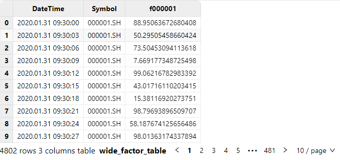
3-second snapshot frequency factor data is used, generating a total of approximately 277GB of data. The data generation script is executed in the DolphinDB client, specifying Datetime and Symbol as partition and sort columns. A partitioned table wide_factor_table is created in the database dfs://test_ai_dataloader. The table includes a Datetime column, a Symbol column for stock names, and 1000 factor columns (named from f000001 to f001000). The types are DATETIME and SYMBOL, with all factor columns of type DOUBLE. The detailed code is found in the project file ddb_scripts.dos. Core code is as follows:
dbName = "dfs://test_ai_dataloader"
tbName = "wide_factor_table"

if (existsDatabase(dbName)) {
    dropDatabase(dbName)
}

// Number of stocks
numSymbols = 250
// Number of factors
numFactors = 1000

dateBegin = 2020.01.01
dateEnd = 2020.01.31
symbolList = symbol(lpad(string(1..numSymbols), 6, "0") + ".SH")
factorList = lpad(string(1..numFactors), 7,"f000000")

colNames = ["Datetime", "Symbol"] join factorList
colTypes = [DATETIME, SYMBOL] join take(DOUBLE, numFactors)
schema = table(1:0, colNames, colTypes)
The following script can be used to check whether the data was successfully written:
select DateTime, Symbol, f000001 from loadTable("dfs://test_ai_dataloader", "wide_factor_table") where Symbol=`000001.SH, date(DateTime)=2020.01.31Example data is as follows:
5.2 PyTorch DataLoader Performance Testing
In traditional deep learning, the following steps are usually used to process training data:
- Generate binary data files.
- Generate index information as a .pkl file.
- Load data into the model using PyTorch's DataLoader.
First, binary data files are generated using the numpy library. This stage takes approximately 83 minutes. Core code is as follows:
st = time.time()
for symbol in symbols:
    for t in times:
        sql_tmp = sql + f""" where Symbol={symbol}, date(DateTime)={t}"""
        data = s.run(sql_tmp, pickleTableToList=True)
        data = np.array(data[2:])
        data.tofile(f"datas/{symbol[1:]}-{t}.bin")
        print(f"[{symbol}-{t}] LOAD OVER {data.shape}")
ed = time.time()
print("total time: ", ed-st)   # Approx. 4950s
During data processing, it is usually necessary to calculate the sliding window size and stride. These two parameters determine how training samples are sliced from the data. The window size defines the temporal length of each training sample, while the stride defines the gap between successive windows. Once the window size and stride are determined, the next step is to calculate which files each sample needs to load data from. This process typically involves iterating through the data and determining slicing based on the window settings. The index information is then stored in index.pkl for later use. This stage takes approximately 4 minutes. Core code is as follows:
with open("index.pkl", 'wb') as f:
    pickle.dump(index_list, f)
ed = time.time()
print("total time: ", ed-st)    # Approx. 234s
Finally, in the Python code, a dataset is defined to manage and load training data. The contents of index.pkl are loaded into memory, and data files are opened using mmap to enable fast access via index. This stage takes approximately 25 minutes. Core code is as follows:
def main():
    torch.set_default_device("cuda")
    torch.set_default_tensor_type(torch.DoubleTensor)

    model = SimpleNet()
    model = model.to("cuda")

    loss_fn = nn.MSELoss()
    loss_fn = loss_fn.to("cuda")
    optimizer = torch.optim.Adam(model.parameters(), lr=0.05)
    dataset = MyDataset(4802)
    dataloader = DataLoader(
        dataset, batch_size=64, shuffle=False, num_workers=3,
        pin_memory=True, pin_memory_device="cuda",
        prefetch_factor=5,
    )

    epoch = 10
    for _ in range(epoch):
        for x, y in tqdm(dataloader, mininterval=1):
            x = x.to("cuda")
            y = y.to("cuda")
            y_pred = model(x)
            loss = loss_fn(y_pred, y)
            optimizer.zero_grad()
            loss.backward()
            optimizer.step()

if __name__ == "__main__":
    main()
At this point, the PyTorch DataLoader-based deep learning training data pipeline is complete. The first stage (generating binary files) takes approximately 83 minutes. The second stage (generating index information) takes 4 minutes. The third stage (20,000 training iterations) takes 25 minutes. The total time is 112 minutes.
5.3 DDBDataLoader Performance Testing
With DDBDataLoader , the following steps are typically used to
process training data:
- Load data from the DolphinDB distributed table.
- Process the loaded data into a format required for training.
In this test, DDBDataLoader is used to fetch training data.
Unlike traditional methods, it does not require saving data to files for
client-side processing. Instead, SQL query results are directly converted into
torch.Tensor via a Session, reducing data transmission and
storage overhead. In the test code, Python's third-party library
line_profiler is used to measure execution time for various
parts, such as data loading and model training. The test steps are as
follows:
Define DDBDataLoader
The following code is executed in the Python client, using an existing database table. SQL query results serve as the dataset. The dataset specifies the target column as ["f000001"], excluding Symbol and DateTime columns.
import dolphindb as ddb
from dolphindb_tools.dataloader import DDBDataLoader

sess = ddb.Session()
sess.connect('localhost', 8848, "admin", "123456")

dbPath = "dfs://test_ai_dataloader"
tbName = "wide_factor_table"

symbols = ["`" + f"{i}.SH".zfill(9) for i in range(1, 251)]
times = ["2020.01." + f"{i+1}".zfill(2) for i in range(31)]

sql = f"""select * from loadTable("{dbPath}", "{tbName}")"""

dataloader = DDBDataLoader(
    s, sql, targetCol=["f000001"], batchSize=64, shuffle=True,
    windowSize=[200, 1], windowStride=[1, 1],
    repartitionCol="date(DateTime)", repartitionScheme=times,
    groupCol="Symbol", groupScheme=symbols,
    seed=0,
    offset=200, excludeCol=["DateTime", "Symbol"], device="cuda",
    prefetchBatch=5, prepartitionNum=3
)
Key parameters explained:
batchSize=64indicates the batch size is 64.windowSize=[200, 1], windowStride=[1, 1], offset=200indicates the input and target window sizes are 200 and 1 respectively, with strides of 1, and an offset of 200.shuffle=Truemeans data shuffling is enabled, using random seedseed=0- To train using each stock's time series data,
groupCol="Symbol"andgroupScheme=symbolsare specified, wheresymbolsis a list of all stock names. - To reduce data partitioning granularity,
repartitionCol="date(DateTime)"andrepartitionScheme=timesare used, wheretimesincludes all dates from 2020.01.01 to 2020.01.31. - Training is performed on GPU by specifying
device="cuda", sotorch.Tensoris created on the GPU. prefetchBatch=5,prepartitionNum=3means 5 batches are prepared in advance, and 3 subquery results are preloaded per partition.
These configurations help improve training efficiency and fully utilize GPU and background threads.
Define Network and Train
The following code, executed in the Python client, defines a simple CNN network
structure, along with the loss function and optimizer. Finally, similar to
torch’s DataLoader, it iterates through the DDBDataLoader to
retrieve and input data into the model for training. Core code is as
follows:
model = SimpleNet()
model = model.to("cuda")
loss_fn = nn.MSELoss()
loss_fn = loss_fn.to("cuda")
optimizer = torch.optim.Adam(model.parameters(), lr=0.05)
num_epochs = 10

model.train()
for epoch in range(num_epochs):
    for X, y in dataloader:
        X = X.to("cuda")
        y = y.to("cuda")
        y_pred = model(X)
        loss = loss_fn(y_pred, y)
        optimizer.zero_grad()
        loss.backward()
        optimizer.step()
By directly converting data to torch.Tensor and using
DDBDataLoader for data management, training data can be
accessed and utilized more efficiently, improving deep learning model training
efficiency. This approach reduces data transmission and storage overhead, and
makes the training process more flexible and efficient. Total time cost for this
method is 25 minutes.
Performance Comparison
This test compares the traditional method (PyTorch DataLoader) and
DDBDataLoader. DDBDataLoader, with
integrated PyTorch support, takes about 25 minutes, uses 0.8 GB memory, and 70
lines of code. In contrast, PyTorch DataLoader takes 112 minutes, 4 GB memory,
and over 200 lines of code. Key reasons include:
- Performance Improvement:
DDBDataLoadersignificantly reduces data preparation and iteration time. It retrieves and shuffles data partitions directly from DolphinDB, avoiding the traditional export-to-disk and re-import workflow that hinders performance. - Increased Flexibility:
DDBDataLoaderinitializes using SQL, allowing high flexibility. Users can create new factors via SQL and immediately apply them in PyTorch training—unlike traditional methods, which require re-exporting data. - Reduced Memory Usage: DolphinDB employs internal parallel threads and
message queues, recycling memory after use. Traditional methods often load
full datasets into memory, leading to long memory residency and risk of OOM.
DDBDataLoaderreduces memory usage to 1/5 of the traditional method. - Reduced Code Complexity: DolphinDB wraps a DataLoader interface with minimal user intervention—only 70 lines of code. The traditional approach needs custom interfaces for dataset and PyTorch integration, totaling over 200 lines. This greatly reduces development and maintenance costs.
In summary, DDBDataLoader can improve performance and
significantly reduce development and operational costs when training PyTorch
models with data stored in DolphinDB.
6. Conclusion
DDBDataLoader represents DolphinDB’s exploration into the
integration of deep learning and database technologies. It is designed to address
the following key challenges:
- It fully leverages the features of DolphinDB by splitting SQL queries into multiple sub-queries, thereby reducing memory usage on the client side.
DDBDataLoaderretrieves data directly from the database through on-demand queries, enabling flexible data operations, improved efficiency, and reduced development and operational costs.
In summary, integrating DolphinDB and DDBDataLoader into the factor
data management workflow helps better meet the needs of quantitative investment
strategies and unlock the full potential of deep learning models. This integration
enhances efficiency, reduces cost, and provides more powerful capabilities for
factor data management and application.